Next: 4 Double-integral Kramers' theory
Up: unfolding_distributions
Previous: 2 Review of current
Subsections
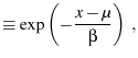
Let  be the end to end distance of the protein,
  be the time since loading began,
  be tension applied to the protein,
  be the surviving population of folded proteins.
Make the definitions
be the surviving population of folded proteins.
Make the definitions
 |
 |
|
the pulling velocity |
(1) |
 |
 |
|
the loading spring constant |
(2) |
 |
 |
|
the initial number of folded proteins |
(3) |
 |
 |
|
the number of dead (unfolded) proteins |
(4) |
 |
 |
|
the unfolding rate |
(5) |
The proteins are under constant loading because
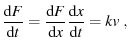 |
(6) |
a constant, since both  and
and  are constant (Evans and Ritchie (1997) in the text on the first page, Dudko et al. (2006) in the text just before Eqn. 4).
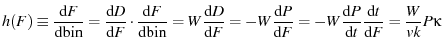
The instantaneous likelyhood of a protein unfolding is given by
 , and the unfolding histogram is merely this function discretized over a bin of width
  (This is similar to Dudko et al. (2006) Eqn. 2, remembering that
 , that their probability density is not a histogram (
 ), and that their pdf is normalized to
  ).
).
 |
(7) |
Solving for theoretical histograms is merely a question of taking your chosen  , solving for
  , and plugging into Eqn. 7.
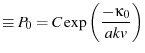
We can also make a bit of progress solving for in terms of as follows:
, and plugging into Eqn. 7.
We can also make a bit of progress solving for in terms of as follows:
where
 is a constant of integration scaling .
In the extremely weak tension regime, the proteins' unfolding rate is independent of tension, we have
Suprise! A constant unfolding-rate/hazard-function gives exponential decay.
Not the most earth shattering result, but it's a comforting first step, and it does show explicitly the dependence in terms of the various unfolding-specific parameters.
Stepping up the intensity a bit, we come to Bell's model for unfolding
(Hummer and Szabo (2003) Eqn. 1 and the first paragraph of Dudko et al. (2006) and Dudko et al. (2007)).
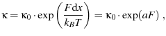 |
(15) |
where we've defined
 to bundle some constants together.
The unfolding histogram is then given by
to bundle some constants together.
The unfolding histogram is then given by
The dependent behavior reduces to
![$\displaystyle h(F) \propto \exp\p[{a F - b\exp(a F)}] \;,$](img46.png) |
(21) |
where
 is
another constant rephrasing.
is
another constant rephrasing.
This looks an awful lot like the the Gompertz/Gumbel/Fisher-Tippett
distribution, where
but we have
 |
(24) |
Strangely, the Gumbel distribution is supposed to derive from an
exponentially increasing hazard function, which is where we started
for our derivation. I haven't been able to find a good explaination
of this discrepancy yet, but I have found a source that echos my
result (Wu et al. (2004) Eqn. 1).
Oh wait, we can do this:
 |
(25) |
with
 . I feel silly... From
Wolframhttp://mathworld.wolfram.com/GumbelDistribution.html,
the mean of the Gumbel probability density
. I feel silly... From
Wolframhttp://mathworld.wolfram.com/GumbelDistribution.html,
the mean of the Gumbel probability density
![$\displaystyle P(x) = \frac{1}{\beta} \exp\p[{\frac{x-\alpha}{\beta} -\exp\p({\frac{x-\alpha}{\beta}}) }]$](img55.png) |
(26) |
is given by
 , and the variance is
 , where
 is
the Euler-Mascheroni constant. Selecting
is
the Euler-Mascheroni constant. Selecting
 ,
,
 , and
, and  we have
 |
![$\displaystyle = \frac{1}{\beta} \exp\p[{\frac{F+\beta\ln(\kappa\beta/kv)}{\beta} -\exp\p({\frac{F+\beta\ln(\kappa\beta/kv)} {\beta}}) }]$](img63.png) |
(27) |
| |
![$\displaystyle = \frac{1}{\beta} \exp(F/\beta)\exp[\ln(\kappa\beta/kv)] \exp\p\{{-\exp(F/\beta)\exp[\ln(\kappa\beta/kv)]}\}$](img64.png) |
(28) |
| |
![$\displaystyle = \frac{1}{\beta} \frac{\kappa\beta}{kv} \exp(F/\beta) \exp\p[{-\kappa\beta/kv\exp(F/\beta)}]$](img65.png) |
(29) |
| |
![$\displaystyle = \frac{\kappa}{kv} \exp(F/\beta)\exp[-\kappa\beta/kv\exp(F/\beta)]$](img66.png) |
(30) |
| |
![$\displaystyle = \frac{\kappa}{kv} \exp(F/\beta - \kappa\beta/kv\exp(F/\beta)]$](img67.png) |
(31) |
| |
![$\displaystyle = \frac{\kappa}{kv} \exp(aF - \kappa/akv\exp(aF)]$](img68.png) |
(32) |
| |
![$\displaystyle = \frac{\kappa}{kv} \exp(aF - b\exp(aF)] \propto h(F) \;.$](img69.png) |
(33) |
So our unfolding force histogram for a single Bell domain under
constant loading does indeed follow the Gumbel distribution.
For the saddle-point approximation for Kramers' model for unfolding
(Evans and Ritchie (1997) Eqn. 3, () Eqn. 4.56c, van Kampen (2007) Eqn. XIII.2.2).
 |
(34) |
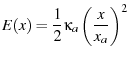
where  is the barrier height under an external force ,
 is the diffusion constant of the protein conformation along the reaction coordinate,
 is the characteristic length of the bound state
 ,
,
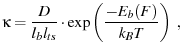
 is the density of states in the bound state, and
 is the characteristic length of the transition state
 |
(35) |
Evans and Ritchie (1997) solved this unfolding rate for both inverse power law potentials and cusp potentials.
 |
(36) |
(e.g.  for a van der Waals interaction, see Evans and Ritchie (1997) in
the text on page 1544, in the first paragraph of the section
Dissociation under force from an inverse power law attraction).
Evans then gets funky with diffusion constants that depend on the
protein's end to end distance, and I haven't worked out the math
yet...
for a van der Waals interaction, see Evans and Ritchie (1997) in
the text on page 1544, in the first paragraph of the section
Dissociation under force from an inverse power law attraction).
Evans then gets funky with diffusion constants that depend on the
protein's end to end distance, and I haven't worked out the math
yet...
 |
(37) |
(see Evans and Ritchie (1997) in the text on page 1545, in the first paragraph
of the section Dissociation under force from a deep harmonic well).
Next: 4 Double-integral Kramers' theory
Up: unfolding_distributions
Previous: 2 Review of current
Download unfolding_distributions.pdf
View the source files or my
.latex2html-init configuration file
3 Single-domain proteins under constant loading
Copyright © 2009-10-12, W. Trevor King
(contact)
Released under the GNU Free Document License, Version 1.2 or later
Drexel Physics


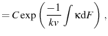
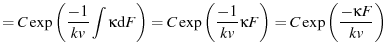
![$\displaystyle = C\exp\p({\frac{-1}{kv}\ensuremath{\int {\kappa} \dd {F}}}) = C\...
...{kv} \frac{\kappa_0}{a} \exp(a F)}] = C\exp\p[{\frac{-\kappa_0}{akv}\exp(a F)}]$](img40.png)
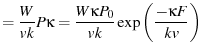
![$\displaystyle = \frac{W}{vk} P \kappa = \frac{W}{vk} P_0 \exp\p\{{\frac{\kappa_...
...\frac{W\kappa_0 P_0}{vk} \exp\p\{{a F + \frac{\kappa_0}{akv}[1-\exp(a F)]}\}\;.$](img45.png)