A More Fundamental Analysis of The Simultaneous Over Relaxation Method

Whereas our principal mathematical justification for an iterative averaging comes from the mean value property, the behavior of the iteration in terms of convergence must ultimately come from the properties of the numerical methods. In this section we will look closer at the mathematical details of our iterative processes with the ultimate goal of finding the optimal SOR coefficient.

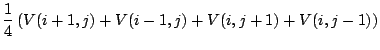
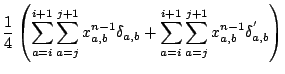
We can generalize the Jacobi method by differentiating for boundary conditions,

$$V(i,j) = \frac{1}{4}\left(V(i+1,j)+V(i-1,j)+V(i,j+1)+V(i,j-1)\right)$$ (3.1)

$$x^n_{i,j} = \frac{1}{4}\left(x^{n-1}_{i+1,j}-x^{n-1}_{i-1,j}-x^{n-1}_{i,j+1}-x^{n-1}_{i,j-1}\right)$$ (3.2)

$$= \frac{1}{4}\left(\sum_{a=i}^{i+1}\sum_{a=j}^{j+1}x^{n-1}_{a,b}\delta_{a,b} + \sum_{a=i}^{i+1}\sum_{a=j}^{j+1}x^{n-1}_{a,b}\delta^{'}_{a,b}\right)$$ (3.3)

Here $\delta$ selects those values which are non-boundary values, and $\delta'$ indicates those which are boundary conditions.

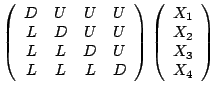
The above equation can be generalized by writing, for the Jacobi case,

$$Dx^{n+1}=Bx^n + b$$ (3.4)

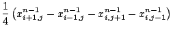
For the GS case, we use the new values as they become available whereby,

$$D(x[k+1])=Lx[k+1]+Ux[k]+b$$

The reader can convince themselves that L is a lower triangular matrix and U an upper triangular, where the Jacobi form could be simplified as, for example,

$$\left(\begin{array}{cccc}D&U&U&U L&D&U&U L&L&D&U L&L&L&D\end{array}\right)\left(\begin{array}{c}X_1 X_2 X_3 X_4\end{array}\right)$$ (3.5)

That L is a triangular matrix and D is uniformly nonzero along the diagonal means that the determinant of D-L will not be zero, whereby D-L is invertible. Thus we have,

$$x[k+1] = (D-L)^{-1}Ux[k] + (D-L)^{-1}b,$$

$$x[k+1] = D^{-1}\left(Lx[k+1]+Ux[k]+b\right)$$ (3.6)

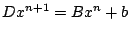
SOR has us calculate the difference between the new value of the potential we are calculating as recommended by GS, and the old value pre-calculation. Calling this difference Q, SOR then adds wQ to the old coefficients, where w is the SOR coefficient to be determined for optimal progress ($w=1$ is simply GS, $w>1$ is SOR). Thus in matrix form, the SOR method can be written

$$x[k+1] = x[k]+w\left(D^{-1}\left(Lx[k+1]+Ux[k]+b\right)-x[k]\right)$$ (3.7)

$$(D-wL)x[k+1] = (1-w)Dx[k]+wUx[k]+wb$$

$$x[k+1] = (D-wL)^{-1}\left((1-w)D+wU\right)x[k]+(D-wL)^{-1}wb$$

And obvious substitution is

$$H = (D-wL)^{-1}\left((1-w)D+wU\right),$$

from which we get

$$x[k+1]=Hx[k]+(D-wL)^{-1}wb$$ (3.8)

The reader is encouraged to view reference [2],[3] for a more detailed exposition, as we take more than a few liberties of omitting detail here.