


Next: The Integration
Up: Detailed Derivation of the
Previous: Assumptions
We assume the system can be modeled with the Hamiltonian,
![$\displaystyle H_{s}=\hbar \omega a^{\dagger}a, \ \ \ [a,a^{\dagger}]=1$](img10.png) |
(2.1) |
Separately we assume that there exists a bath which can be
modeled with the Hamiltonian,
![$\displaystyle H_{b}=\sum_i \hbar \omega_i b_i^{\dagger}b_i, \ \ \ [b_i,b_k^{\dagger}]=\delta_{ik}$](img11.png) |
(2.2) |
Finally, as stated before, the interaction of the bath and system is
taken in the form of
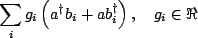 |
(2.3) |
The total Hamiltonian is,
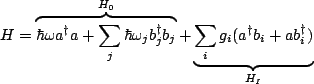 |
(2.4) |
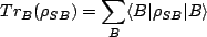
We assume uncertainty in the preparation of states, so we switch to the
density operator regime. We call the density operator corresponding to our bath coupled system  (S: Single original oscillator; B: Environment) where the individual density operators can be retrieved via a trace, i.e.
 |
 |
 Trace over environment states Trace over environment states |
|
 |
|
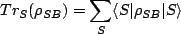 Trace over local states Trace over local states |
|
The dynamics of the system evolve as (Liouville equation),
![$\displaystyle i\hbar\frac{d\rho_{SE}}{dt}=[H,\rho_{SE}]$](img20.png) |
(2.5) |
We commit a unitary transform to simplify this equation as follows (the so-called interaction picture). It can be shown that,
![$\displaystyle \exp(\alpha A)B\exp(-\alpha A)= B + \alpha[A,B] + \frac{\alpha^2}{2!}[A,[A,B]] + \cdots$](img21.png) |
(2.6) |
Furthermore, from the premises of Quantum Mechanics, it is legitimate to commit
transforms of the type,
 Unitary Unitary |
(2.7) |
These so called similarity transformations preserve rank, determinant, trace, and eigenvalues.
We let,
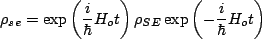 |
(2.8) |
We take the time derivative and find,
![$\displaystyle \frac{d\rho_{se}}{dt}=\frac{i}{\hbar}[H_o,\rho_{se}]-\frac{i}{\hb...
...(\frac{i}{\hbar}H_o t\right)[H,\rho_{SE}]\exp\left(-\frac{i}{\hbar}H_o t\right)$](img24.png) |
(2.9) |
From equation 2.6, since
and
![$ [H_o,H_o] = 0$](img26.png) ,
,
![$\displaystyle \frac{d\rho_{se}}{dt}=-\frac{i}{\hbar}[H_i, \rho_{se}]$](img28.png) |
(2.10) |
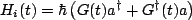
where  is the transform of
  and can be calculated as follows. We know that,
and whereas
and can be calculated as follows. We know that,
and whereas
 , equation 2.6 gives
can be calculated in this fashion for both the
 and the multiple set
 ,
where it is thus now trivial to find that,
,
where it is thus now trivial to find that,
 |
(2.11) |
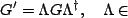
If we now define
we can simplify to
 |
(2.12) |
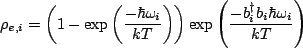
Since the bath is in equilibrium, we can construct  easily. Let
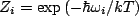 . Then the probability that one
mode (i) of the field is excited with n photons is
. Then the probability that one
mode (i) of the field is excited with n photons is
 |
(2.13) |
The density matrix for this mode is then
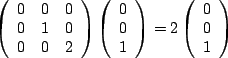
To simplify this further, we imagine a three states system in which we can represent
 as,
for example letting
as,
for example letting  ,
The above sum could then be written,
We recover the matrix, and so we can write just as well,
,
The above sum could then be written,
We recover the matrix, and so we can write just as well,
 |
(2.15) |
By the rules of probability, the density operator for the entire bath becomes,
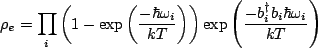 |
(2.16) |
By our assumptions, this is the state of the bath for all time, and so we will not write this as a function of time. The form  will take will be much more complicated, and it is the purpose of this report to derive the differential equation defining its time evolution.
Next: The Integration
Up: Detailed Derivation of the
Previous: Assumptions
Timothy Jones
2006-10-11
![$\displaystyle 0\left(\begin{array}{c}1\\ 0\\ 0\end{array}\right)\left[\begin{ar...
...y}{c}0\\ 0\\ 1\end{array}\right)\left[\begin{array}{ccc}0&0&1\end{array}\right]$](img51.png)