From the Hydrogenic: The Aufbau Prinicipal

Though we demonstrated the basic theory of the hydrogen atom in previous sections, we now wish to consider a simple model for more complex atoms. An atom with atomic number Z, i.e. Z protons, if it is neutral, will have Z matching electrons whereby we might write the Hamiltonian as,

$$H = \sum^Z_{j=1}\left(-\frac{-\hbar^2}{2m}\nabla^2_j - \left(\fra... ...frac{1}{4\pi \epsilon_0}\right)\sum^Z_{j\neq k}\frac{e^2}{\vert r_j - r_k\vert}$$ (1.1)

A simple model for hydrogenic atoms invokes the Aufbau principal, of building up atoms from the hydrogen case. We know that the electron requires anti-symetric wave functions, and a generally (though not completely) accurate set of rules called Hund's Rules give us a good guide for ``building'' up the other atoms from hydrogen, namely:

• States with larger S lie lower
• For an S state, the higher the L, the lower the energy
• For any L and S, if the shell is less than half-filled, the lower state has $J=\vert L-S\vert$ , else the lower state is $J=L+S$ .

Gilmore and Jones have produced a periodic table that demonstrates this shell filling model (though it ignores the exceptional cases for simplicity) that is reproduced on in Figure 1. A completely filled shell is much less reactive (has larger ionization binding energy) than a nearly empty shell (the Alkali metals for example), and so the latter type are useful for many optical experiments.

We are particulary interested in atoms which have very hydrogenic properties and whose outer most electron (typically, an Alkali metal with only one valence electron) is in a state with an extremely highh principal quantum number $n\geq 50$ . Rubidium is a common example. (In the experiments done on trapped ions at the National Institute of Standards and Technology, positively ionized Beryllium is used. The ionization is necessary for trapping; and the missing valance electron leaves the ion with only one valance. However, the ion need not be in the Rydberg state for these experiments).

Here we briefly survey the systematic way in which the periodic table is built up (Aufbau). We demonstrate a system this author uses to simplify the process of spectral identification of elements, where the spectral identification is recorded as $^{2S+1}L_J$ . Here the capital letters are used to indicate we are dealing with totals.

Figure 1.1: General order of energy levels in the Aufbau buildup process

From Figure 1 we have the following rules for energy level buildup (excluding the 1s starter). Here we start from the bottom right, work our way diagonally through the shells, and then loop back to the next diagonal circuit. We find:

1. Every n level will starts off exactly two loops.
2. Each l value starts off two loops as well, with a higher n for the second case.
3. Following the diagonal, the l value decreases as n increases so that their binary sum is exactly equal to the given loop.

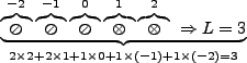
We also need use of binary addition, where the number five is written, for example, as:

$$\underbrace{1}_{2^2}\underbrace{1}_{2_1}\underbrace{0}_{2_0} = 1 \times 4 + 1 \times 2 + 0 \times 1 = 5$$

With these rules, as well as Hund's rules, we can identify the elements. The system is introduced by examples. Our first element is Hydrogen (Z=1), with a single (1s) shell filled. We thus write this as,

$$\overbrace{1}^Z-\overbrace{001}^{n=1}-\overbrace{000}^{l=0}-\overbrace{\oslash}^{\mbox{Shell half-filled}} \ \Rightarrow \ (1s) \ : \ ^2S_{1/2}$$

Here, $l=0$ so our main label is S. There is one unpaired electron, so that our spin is 1/2, whereby we have $^2S$ . Finally, the shell is at least half filled, so our J is additive, and we have $^2S_{1/2}$ .

Next we have Helium, and we finish filling the 1s shell:

$$\overbrace{2}^Z-\overbrace{001}^{n=1}-\overbrace{000}^{l=0}-\overbrace{\otimes}^{\mbox{Shell filled}} \ \Rightarrow \ (1s)^2 \ : \ ^1S_{0}$$

In this case, the shell is completely filled (the ionization energy is at a maxium for this loop) so we have no unpaired electrons (the Pauli exclusion principal demands that a filled shell unit will have one spin up and one spin down electron) and total spin is zero.

Now that the (1s) shell is filled, and our loop takes us the $n=2$ level with Lithium,

$$\overbrace{2}^Z-\overbrace{010}^{n=2}-\overbrace{000}^{l=0}-\over... ...e{\oslash}^{\mbox{Shell half-filled}} \ \Rightarrow \ (He)(2s) \ : \ ^2S_{1/2}$$

Once we get to the third loop, $l=1$ and we have three shells to fill (corresponding to $m=0,\pm 1$ ). For example,

$$\overbrace{2}^Z-\overbrace{010}^{n=2}-\overbrace{001}^{l=1}-\over... ...s}^{\mbox{Shell $<$\ 1/2 filled}} \ \Rightarrow \ He(2s)^2(2p) \ : \ ^2P_{1/2}$$

Here the shell is less than half filled, so $J=\vert L-S\vert=1/2$ .

How do we account for the total angular momentum? Based on Hund's rule that higher l corresponds to lower energy, we consider an amendment to the system that takes account of the vectoral addition of l such that we match the convention. For any set of subshells, the center shell corresponds to zero, the rightward shells correspond to increasing levels of l, and the leftward decreasing levels from zero. Consider,for example, Sc, Z = 21, whose shells will fill as

$$\overbrace{\circ}^{-2}\overbrace{\circ}^{-1}\overbrace{\circ}^{0}\overbrace{\circ}^{1}\overbrace{\oslash}^{2} \ \Rightarrow L = 2$$

Mn as another example gives,

$$\overbrace{\oslash}^{-2}\overbrace{\oslash}^{-1}\overbrace{\oslash}^{0}\overbrace{\oslash}^{1}\overbrace{\oslash}^{2} \ \Rightarrow L = 0$$

While Co has,

$$\underbrace{\overbrace{\oslash}^{-2}\overbrace{\oslash}^{-1}\over... ...L = 3}_{2\times2 + 2 \times 1 + 1 \times 0 + 1 \times (-1) + 1 \times (-2) = 3}$$

Of course, there are exceptions such as Cr, where we would expect,

$$\overbrace{\circ}^{-2}\overbrace{\oslash}^{-1}\overbrace{\oslash}^{0}\overbrace{\oslash}^{1}\overbrace{\oslash}^{2} \ \Rightarrow L = 2$$

It so happens, though, that Cr works out to have $L=0$ . This methodology has the benefit of being systematic enough to lend to easy comprehension, once the user gets used to the rules. As well, once could quite easily program these rules into a computer to output a generalized table. We present a partial list of the periodic table (the first three loops) as a final example.

Loop	Z	*n* - *l* - *shell*	Shell	Code
1	1	$001-000-\oslash$	$(1s)$	$^2S_{1/2}$
	2	$001-000-\otimes$	$(1s)^2$	$^1S_{0}$
2	3	$010-000-\oslash$	$(He)(2s)$	$^2S_{1/2}$
	4	$010-000-\otimes$	$(He)(2s)^2$	$^1S_{0}$
3	5	$010-001-\circ \circ \oslash$	$(He)(2s)^2(2p)$	$^2P_{1/2}$
	6	$010-001-\circ \oslash \oslash$	$(He)(2s)^2(2p)^2$	$^3P_{0}$
	7	$010-001-\oslash \oslash \oslash$	$(He)(2s)^2(2p)^3$	$^4S_{3/2}$
	8	$010-001-\oslash \oslash \otimes$	$(He)(2s)^2 (2p)^4$	$^3P_{2}$
	9	$010-001-\oslash \otimes \otimes$	$(He)(2s)^2 (2p)^5$	$^2P_{3/2}$
	10	$010-001-\otimes \otimes \otimes$	$(He)(2s)^2 (2p)^6$	$^1S_{0}$
	11	$011-000-\oslash$	$Ne(3s)$	$^2S_{1/2}$
	12	$011-000-\otimes$	$Ne(3s)^2$	$^1S_{0}$