Next: Technical details
Up: Activation of the equation
Previous: Kapitsa's Secular Approximation
For a more formal analysis refer to [6].
Starting with the equation,
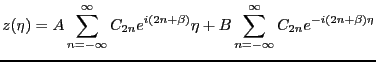
We apply Floquet's theorem and the subsequent corollary to suppose solutions of the form,
The conditions for stability require that  be purely imaginary. It is typical to
write
be purely imaginary. It is typical to
write
 , and so we can take a fourier expansion of the
  , and recalling that the original equation contains
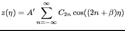
 , we assume a general solution,
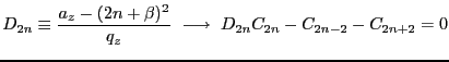
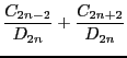
As before, we can find a useful recurssion relation. Define:
When  we have
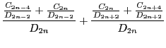
With this recurssion relationship we may solve for  with
increasing levels of accuracy, for example,
with
increasing levels of accuracy, for example,
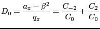
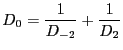
As a first approximation, we set
 and obtain
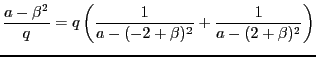
When we assume
 we obtain the approximation,
If we take
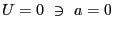 then we find we have recovered the
approximation of the previous section,
then we find we have recovered the
approximation of the previous section,
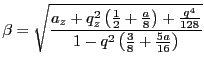
From such references as [8] we know that the next approxmation
is
The motion will have frequencies of
 , of which
the lowest and second to the lowest correspond roughly with the secular
approximation secular and micromotion.
We could carry this process on ad infinitum ad nauseum. This is but one
method to solve for
. The other method is the numerical method
we used to find the stable points of the iso-
. A third method is to use the
more technical solutions to the Mathieu equation devoloped by the
mathematicians. We will close this report with a brief review of one
such solution.
, of which
the lowest and second to the lowest correspond roughly with the secular
approximation secular and micromotion.
We could carry this process on ad infinitum ad nauseum. This is but one
method to solve for
. The other method is the numerical method
we used to find the stable points of the iso-
. A third method is to use the
more technical solutions to the Mathieu equation devoloped by the
mathematicians. We will close this report with a brief review of one
such solution.
Next: Technical details
Up: Activation of the equation
Previous: Kapitsa's Secular Approximation
tim jones
2008-07-07