


Next: A solution with Mathieu's
Up: Activation of the equation
Previous: Activation of the equation
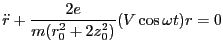
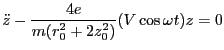
We neglect the DC potential U for now and assume the equations
of motion are of the form, for the rf Paul Ideal chamber ion trap:
 |
|
|
|
 |
|
|
(4.1) |
Define
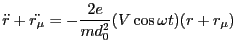
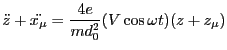
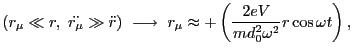
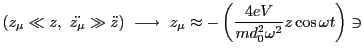
 . Assume that the r and z motion can
be partitioned into large-amp slow ``secular'' motion r and z, and
small-amp high frequency micromotion
. Assume that the r and z motion can
be partitioned into large-amp slow ``secular'' motion r and z, and
small-amp high frequency micromotion  ,
,  at the frequency
of the applied potential
at the frequency
of the applied potential  . Then our equations become
 |
|
|
|
 |
|
|
(4.2) |
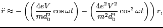
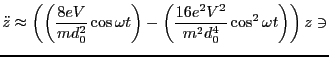
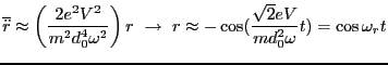
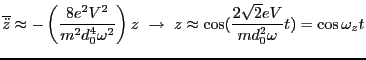
Evidently,
 . We can thus write,
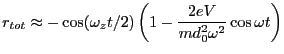
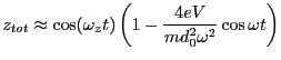
The results of these approximations are graphically displayed in Figures 4.1 and 4.2
created with the following C code:
  float w=53;
  float wz=4;
  float r,z;
  float t=0.0;
  while(t<1000){
  r=-cos(wz*t/2)*(1-0.3*cos(w*t));
  z=cos(wz*t)*(1-0.6*cos(w*t));
  t+=0.01;}
Figure 4.1:
Secular approximation time series
|
|
Figure 4.2:
Secular approximation orbits
|
|
Next: A solution with Mathieu's
Up: Activation of the equation
Previous: Activation of the equation
tim jones
2008-07-07
![\includegraphics[width=6cm]{liss2.ps}](img113.png)
![\includegraphics[width=6cm]{liss.ps}](img114.png)