 |
(2.10) |
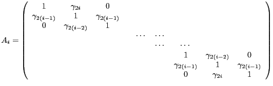
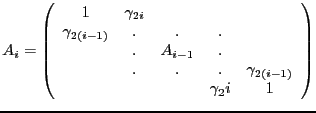
We have
![]() We can
decompose
We can
decompose ![]() in terms of
in terms of ![]() ,
,
 |
(2.11) |
 |
(2.12) |
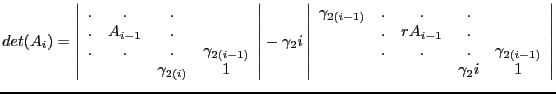
so that
 det
detand

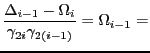
Plugging this into Equation 2.13,
Define
Maple finds,
with(linalg):
C:=matrix([[1,e6,0,0,0,0,0],[e4,1,e4,0,0,0,0],[0,e2,1,e2,0,0,0],
   [0,0,e0,1,e0,0,0],[0,0,0,e2,1,e2,0],[0,0,0,0,e4,1,e4],[0,0,0,0,0,e6,1]]):
dc:=det(C);
dc := -2*e2^2*e0*e4^2*e6+e2^2*e4^2-2*e4^2*e2*e0*e6^2+2*e2*e4^2*e6
       +e4^2*e6^2+2*e2^2*e0*e4+4*e2*e0*e6*e4-2*e2*e4-2*e6*e4-2*e2*e0+1


A:= matrix([[1,e4,0,0,0],[e2,1,e2,0,0],[0,e0,1,e0,0],
                                               [0,0,e2,1,e2],[0,0,0,e4,1]]):
da:=det(A);
da := 1-2*e2*e4-2*e2*e0+2*e2^2*e0*e4+e2^2*e4^2


B:=matrix([[1,e2,0],[e0,1,e0],[0,e2,1]]):
db:=det(B);
db := 1-2*e2*e0
Our program seeks to find all stable values of ![]() ,
i.e. those that satisfy Equation 2.9 as real
values (i.e. all iso-
,
i.e. those that satisfy Equation 2.9 as real
values (i.e. all iso-![]() for which
for which ![]() is exclusively
imaginary.
is exclusively
imaginary.
Our code finds all such iso-![]() by looping through
the a and q axis. If our
by looping through
the a and q axis. If our ![]() formula returns ``nan''
which is the C language's way of saying not a real number,
then we set the value of
formula returns ``nan''
which is the C language's way of saying not a real number,
then we set the value of ![]() to zero, though of course
it is only the imaginary part of
to zero, though of course
it is only the imaginary part of ![]() which is actually
zero. We perform a contour plot on our data output and find
the elegant avian like image of the stability region of
Mathieu's equation (Figure 2.1).
which is actually
zero. We perform a contour plot on our data output and find
the elegant avian like image of the stability region of
Mathieu's equation (Figure 2.1).
For the quadropole field, the rf linear Paul trap,
we have the following stability regime (Figure 2.2). The original
stability diagram is simply reflected about the x-axis as
![]() between the two.
between the two.
![\includegraphics[width=7.5cm]{stable8.ps}](img92.png)
|
![\includegraphics[width=7.5cm]{rf2.ps}](img93.png)
|
For the chamber rf Paul trap, we recall that for
the z direction we must allow for
![]() (Equation 1.3), and so the lowest region of stability (and the largest region at that) has
a slightly different look (Figure 2.4).
(Equation 1.3), and so the lowest region of stability (and the largest region at that) has
a slightly different look (Figure 2.4).
![\includegraphics[width=10cm]{rf4.ps}](img95.png)
|
![\includegraphics[width=7.5cm]{stable5.ps}](img91.png)