


Next: Conclusion
Up: Is Quantum Decoherence the
Previous: Theoretical Example of Decoherence
Contents
We now engage the full apparatus seen in Figure 3.1. The cavity (C) is loaded with a coherent field that is off
resonance with the
 transition frequency but instead is tuned close to a seperate transition (
 transition (n=52, 48.180 GHz)). The cavity is designed so that the atom traverses
the field adiabatically [3]. An atom in the state
transition (n=52, 48.180 GHz)). The cavity is designed so that the atom traverses
the field adiabatically [3]. An atom in the state  will thus interact with this
field, and so we need to consider the full quantum case of Rabi oscillation as the phase of the coherent cavity
field will be shifted. However, the principle is the same as in the semi-classical case, so that we simply state the result. The coherent field will be phase shifted by the presence of any atom in the
state.
will thus interact with this
field, and so we need to consider the full quantum case of Rabi oscillation as the phase of the coherent cavity
field will be shifted. However, the principle is the same as in the semi-classical case, so that we simply state the result. The coherent field will be phase shifted by the presence of any atom in the
state.
After leaving R1, the atom is in the state
 |
(5.1) |
It passes through (C) adiabatically so that no exchange of photons is allowed.
However, the coherent field
 in the chamber will be
phased shifted if the atom is in state
, and as before, a proper
selection of experimental variables and
atomic velocity (
in the chamber will be
phased shifted if the atom is in state
, and as before, a proper
selection of experimental variables and
atomic velocity (
 [3]) can bring this
shift into a particular value (
[3]) can bring this
shift into a particular value ( in this case). More generally (which we
will follow in the dissipation case) the phase shift is
in this case). More generally (which we
will follow in the dissipation case) the phase shift is
 .
.
Thus the field and atom become entangled after passage, i.e.,
 |
(5.2) |
As before, the atom now passes through R2 where it undergoes an  pulse such that the state becomes,
 |
(5.3) |
The field state is now entangled (in a coherent superposition) so that a
measurement of the atom (finding it in either
or  )
will ``project'' the field into the state,
)
will ``project'' the field into the state,
Next we send in a second atom. We assume that this second atom is sent in quickly enough (a time T later)
after the first that relaxation can be neglected. After the second atom passes R1, the
system state is given as (taking the normalization factor as  for simplicity),
The density operator with decay and decoherence will be,
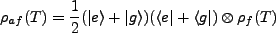 |
(5.4) |
Here  is the density operator of the field which has undergone the decay and decoherence
introduced in the previous section, i.e.
is the density operator of the field which has undergone the decay and decoherence
introduced in the previous section, i.e.
In cavity (C), the atom becomes entangled with the field so that we can write in the non-decay case,
 |
(5.5) |
The decayed density matrix is,
Next the atom passes through R2 and the wave function becomes,
With decay, the density matrix is,
Following Davidovich et al., we write the probability of finding the second atom in
or
as
Since  corresponds to the first atom being detected in the ground state, and
  corresponds
to the first atom being detected in the excited state, one can calculate
corresponds
to the first atom being detected in the excited state, one can calculate  ,
,  , and so on.
Davidovich et al., for example, plot P(g,e,T) and P(e,e,T) as shown in Figure 5.1.
, and so on.
Davidovich et al., for example, plot P(g,e,T) and P(e,e,T) as shown in Figure 5.1.
Figure:
Probabilities of detecting second atom in state
depending on initial state of the first atom (numerical from [3]). Initial decay is decoherence effect. Plateau at 0.5 is classical like-state. Decay at large T corresponds
to relaxation of system into the ground state (
 as
as
 .)
.)
|
|
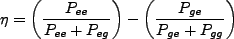
An experiment testing these predictions was first carried out in 1996 by the Paris team [1]. Based
on these theoretical predictions, this team measured the average conditional probability, i.e.
 |
(5.8) |
They find strong agreement with theoretical predictions, as seen in Figure 5.2.
Figure 5.2:
Correlation signal decay due to decoherence. The top line and bottom line represents different
phases induced by different detuning in the (C) chamber. The dashed line corresponds to a higher detuning
and thus a less intefered state and decoheres slower accordingly. Circles and triangles correspond to
experimental results.
 and T is varied. See [1] for details.
|
|
Next: Conclusion
Up: Is Quantum Decoherence the
Previous: Theoretical Example of Decoherence
Contents
tim jones
2007-04-11
![\includegraphics[width=6.0cm]{pee.ps}](img220.png)
![\includegraphics[width=6.0cm]{last.ps}](img222.png)