Next: Experimental Example of Decoherence
Up: Is Quantum Decoherence the
Previous: Experimental Example of Superposition
Contents
We now note that the conditions we have thus far considered are highly artificial. What if we consider
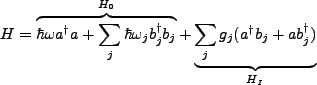
an interaction with the environment? A simple model for an environmental Hamiltonian might be a set of harmonic oscillators,
As developed elsewhere, we can write the interaction Hamiltonian as
A reasonable way to look at this is to see that if the field gains a photon (
 ) then the
single oscillator should loose one
) then the
single oscillator should loose one  and vice versa; the prefactor
  is a coupling constant that
will generally depend on the specifics of the system. The system is now governed by the total Hamiltonian,
is a coupling constant that
will generally depend on the specifics of the system. The system is now governed by the total Hamiltonian,
Let us call the new density operator corresponding to our environmentally coupled system  (S: Single original
oscillator; E: Environment) where the individual density operators can be retrieved via a trace, i.e.
(S: Single original
oscillator; E: Environment) where the individual density operators can be retrieved via a trace, i.e.
 |
 |
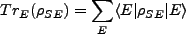 Trace over environment states Trace over environment states |
|
 |
|
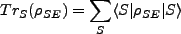 Trace over local states Trace over local states |
|
The dynamics of the system evolve as (Liouville equation),
![$\displaystyle i\hbar\frac{d\rho_{SE}}{dt}=[H,\rho_{SE}]$](img116.png) |
(4.1) |
We commit a unitary transform to simplify this equation as follows (the so-called interaction picture).
Let
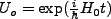 , then
We can then easily find that (since
![$ [H_0, H_0]=0$](img119.png) , letting
, letting
 ),
),
With
 , it is demonstrable that,
And so we have,
 |
(4.4) |
We now follow Orszag and, avoiding some complicated calculations, present a path to the so called master equation[8].
Equation 4.2 is integrated and then reapplied to yield,
![$\displaystyle \frac{d\rho_{se}}{dt}=\frac{1}{i\hbar}[H_i,\rho_{se}(0)]-\frac{1}{\hbar^2}\int^t_0[H_i(t'),[H_i(t'),\rho_{se}(t')]]dt'$](img130.png) |
(4.5) |
It is typically not a bad approximation to assume that the
environment (bath) is large enough to be unperturbed by the
local system, i.e. we assume that (Markovian assumption):
It follows that
Taking the trace of the Equation 4.5 gives,
![$\displaystyle \frac{d\rho_{s}}{dt}=-i \Delta \omega [a^{\dagger}a, \rho_s(t)] +...
...]+A[a\rho_s(t),a^{\dagger}]+B[a^{\dagger},\rho_s(t)a]+B[a^{\dagger}\rho_s(t),a]$](img133.png) |
(4.6) |
Here,
Let
 . The master equation becomes
![$\displaystyle \frac{d\rho_s}{dt}=-i \Delta \omega [a^{\dagger}a, \rho_s(t)]
-\f...
...}a\rho_s(t)-2a\rho_s(t)a^{\dagger}) - \frac{\gamma}{2}\langle n(\omega)\rangle($](img147.png) c.c. c.c. |
(4.7) |
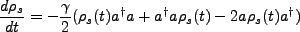
We simplify things even further by considering only the simplest of
baths, where  thus
thus
 , and the master equation is simply
 |
(4.8) |
Now we are ready to examine the evolution of our simple model. We recall
that it was  which Decoherence need destroy to produce the classical
state of
which Decoherence need destroy to produce the classical
state of  . We now apply the master equation to this system and
see what happens to these off-diagonal terms.
. We now apply the master equation to this system and
see what happens to these off-diagonal terms.
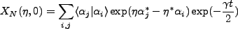
Conventionally, we start with the so-called normally ordered characteristic
function,
We take the time derivative of this function, and using the property
producing [8,9]
The solution to this equation is of the form
Where
 .
Finding our initial conditions as
.
Finding our initial conditions as
It then follows that,
 |
(4.13) |
Now it is time to note that since
And thus,
and
 , the density matrix becomes,
 |
(4.14) |
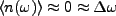
When
 we can approximate the prefactor on the cross terms by
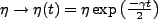
 . It is conventional
to define
. It is conventional
to define
 so that, along with the condition that
 , our
interference term becomes,
, our
interference term becomes,
 |
(4.15) |
In terms of the density matrix,
The diagonal states will decay into the ground state as they reach equilibrium with the bath. However, this decay will generally
be much slower than the decoherence. Finally we must note that decoherence has brought us into a classical density matrix,
but the question still remains about which state we will find the particle in when an actual measurement is taken.
We summarize that decoherence is that part of dampening, caused
by a coupling to an environment, which produces a decay (a stronger
decay) of off-diagonal elements of a density matrix. Thus, in short
time, the local quantum density matrix assumes a classical appearance. Since Decoherence is much quicker than
normal dissipation, it has become a major engineering problem in the search for a quantum computer.
Next: Experimental Example of Decoherence
Up: Is Quantum Decoherence the
Previous: Experimental Example of Superposition
Contents
tim jones
2007-04-11