Next: Quantization of an electromagnetic
Up: A Brief Introduction to
Previous: Gauges
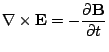
Maxwell's equations for a source free environment are
In this environment,  and
and

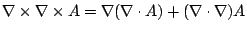
The simplicity of these four equations begs for even further simplification,
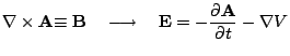
whereby we introduce the vector potential,
There are many ways to fit these equations while maintaining the validity
of the Maxwell equations. The coulomb potential suffices and is preferrable
due to its simplicity:
 ,
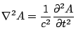
,  . The identity
 coupled with our previous assertation and equation 3 above yield
 |
(3.4) |
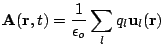
We will quantize this centralized magnetic potential. To completely specify
the field we would have to describe its values for all points in space; it
is customary to develop the quantization in a theoretical cube, and then
let the volume of the cube expand to infinity to accomplish a full discription.
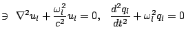
Our derivation can consider standing or plane waves. The case of standing
waves is quicker. We assume the magnetic potential has a solution of form
 |
(3.5) |
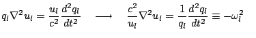
Under this seperation of variables,
 |
|
|
(3.6) |
 |
|
|
(3.7) |
Being in the standing wave regime, there can be no currents on the boundary, implying that
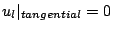 and
and
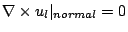 . But of course, we have already
doomed ourselves to the fact that
. But of course, we have already
doomed ourselves to the fact that
 . These consequences become important
as follows.
. These consequences become important
as follows.
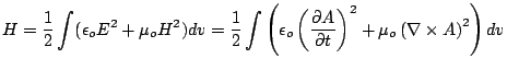
The energy stored by our electromagnetic field is
 |
(3.8) |
We assume via our target solution that our spatial modes will have the orthogonality
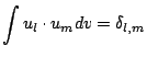 |
(3.9) |
Using this orthogonality, we have
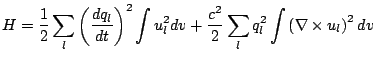 |
(3.10) |
The rightmost integral can be taken with an algebraic manipulation. We examine it as follows:
A snap shot of the latter yields:
This suggest the generating equation
Thus our vector identity is
More appropriate for our needs, we rearrange the previous equation to find:
Reidentifying  and
and
 , we have
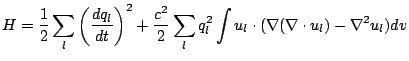
Remembering that this is under a volume integral, we quickly see that the first term Stokes away as a surface
integral which our previously established boundary conditions founded as zero. The second term is taken
care of by the use of a previous vector identity. Catching up, we have
, we have
Remembering that this is under a volume integral, we quickly see that the first term Stokes away as a surface
integral which our previously established boundary conditions founded as zero. The second term is taken
care of by the use of a previous vector identity. Catching up, we have
 |
(3.11) |
With equation 7 and our boundary conditions, this becomes,
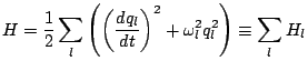 |
(3.12) |
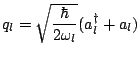
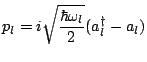
This form is fully equivalant to the harmonic oscillator, and with the following set:
we complete the standing wave quantization by concluding that
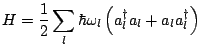 |
(3.16) |
Next: Quantization of an electromagnetic
Up: A Brief Introduction to
Previous: Gauges
Timothy Jones
2006-05-30