The Spherical Harmonic Oscillator

Next we consider the solution for the three dimensional harmonic oscillator in spherical coordinates.

It is obvious that our solution in Cartesian coordinates is simply,

$$E=\hbar\omega \left(n_x + n_y + n_z + \frac{3}{2}\right)$$ (3.1)

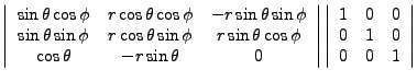
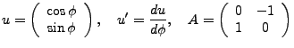
Less simple, but more edifying is the case in spherical coordinates. With the conversions,

$$x=r\sin\theta\cos\phi$$

$$y=r\sin\theta\sin\phi$$

$$z=r\cos\theta$$ (3.2)

we have,

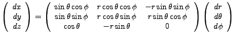$$\left(\begin{array}{c}dx \\ dy\\ dz\end{array}\right)=\left(\begi... ... \end{array}\right)\left(\begin{array}{c}dr\\ d\theta\\ d\phi\end{array}\right)$$ (3.3)

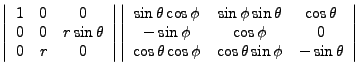
We invert the matrix,

$$\left\vert\begin{array}{ccc}\sin\theta\cos\phi & r\cos\theta\cos\... ...ert\begin{array}{ccc}1 & 0 & 0 \\ 0 & 1 & 0 \\ 0 & 0 & 1 \end{array}\right\vert$$

$$\left\vert\begin{array}{ccc}1 & 0 & 0\\ 0 & 0 & r\sin\theta\\ 0... ...\\ \cos\theta\cos\phi & \cos\theta\sin\phi & -\sin\theta \end{array}\right\vert$$

Thus,

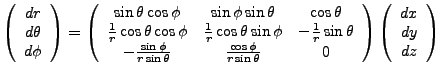$$\left(\begin{array}{c}dr\\ d\theta\\ d\phi\end{array}\right)=\lef... ...eta} & 0 \end{array}\right)\left(\begin{array}{c}dx\\ dy\\ dz\end{array}\right)$$ (3.4)

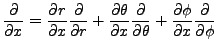
Of course,

$$\frac{\partial}{\partial x}=\frac{\partial r}{\partial x}\frac{\p... ...partial \theta}+ \frac{\partial \phi}{\partial x}\frac{\partial}{\partial \phi}$$

So we also have,

$$\left(\begin{array}{c}\frac{\partial}{\partial x} \\ \frac{\parti... ...c{\partial}{\partial \theta}\\ \frac{\partial}{\partial \phi}\end{array}\right)$$ (3.5)

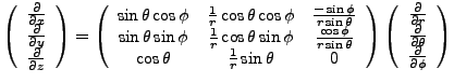
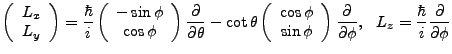
Here we begin an aside on the angular momentum operators. This will be useful because it will bring us half the solution. We have,

$$\left(\begin{array}{c}L_x\\ L_y\\ L_z\end{array}\right)=\left(\be... ...\ \frac{\partial}{\partial y} \\ \frac{\partial}{\partial z} \end{array}\right)$$ (3.6)

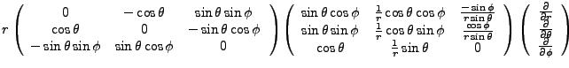
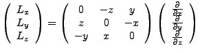
We convert this,

$$r\left(\begin{array}{ccc}0&-\cos\theta&\sin\theta\sin\phi\\ \cos\... ...c{\partial}{\partial \theta}\\ \frac{\partial}{\partial \phi}\end{array}\right)$$

We let

$$u = \left(\begin{array}{c}\cos\phi\\ \sin\phi\end{array}\right),\... ...frac{du}{d\phi}, \ \ \ A = \left(\begin{array}{cc}0&-1\\ 1&0 \end{array}\right)$$

We quickly note that $Au=u'$ and u and u' are orthogonal, so we have:

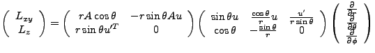$$\left(\begin{array}{c}L_{xy}\\ L_z\end{array}\right)=\left(\begin... ...c{\partial}{\partial \theta}\\ \frac{\partial}{\partial \phi}\end{array}\right)$$ (3.7)

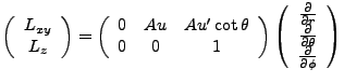$$\left(\begin{array}{c}L_{xy}\\ L_z\end{array}\right)=\left(\begin... ...c{\partial}{\partial \theta}\\ \frac{\partial}{\partial \phi}\end{array}\right)$$ (3.8)

Properly, none of the terms involves $\partial r$. Throwing in the proper $\frac{\hbar}{i}$ we find,

$$\left(\begin{array}{c}L_x\\ L_y\end{array}\right)=\frac{\hbar}{i}... ...artial}{\partial \phi}, \ \ L_z = \frac{\hbar}{i}\frac{\partial}{\partial \phi}$$ (3.9)

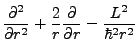
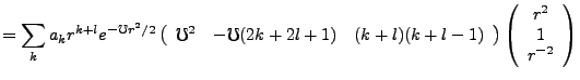
With some algebra we can show that

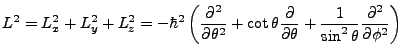$$L^2 = L_x^2 + L_y^2 + L_z^2 = -\hbar^2\left(\frac{\partial^2}{\pa... ...rtial \theta} + \frac{1}{\sin^2\theta}\frac{\partial^2}{\partial \phi^2}\right)$$ (3.10)

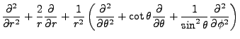
We know that 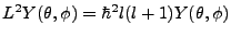$L^2 Y(\theta,\phi)=\hbar^2 l(l+1)Y(\theta,\phi)$. We also have that the Laplacian in spherical coordinates is,

$$\nabla^2 = \frac{\partial^2}{\partial r^2} + \frac{2}{r}\frac{\partial}{\par... ...tial \theta} + \frac{1}{\sin^2\theta}\frac{\partial ^2}{\partial \phi^2}\right)$$

$$\nabla^2 = \frac{\partial^2}{\partial r^2} + \frac{2}{r}\frac{\partial}{\partial r} - \frac{L^2}{\hbar^2 r^2}\right)$$

Thus, in three dimensions and spherical coordinates, the Schrödinger equation is,

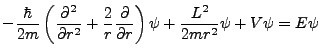$$-\frac{\hbar}{2m}\left(\frac{\partial^2}{\partial r^2} + \frac{2}{r}\frac{\partial}{\partial r}\right)\psi + \frac{L^2}{2mr^2}\psi +V\psi = E \psi$$ (3.11)

By separation of variables, the radial term and the angular term can be divorced. The solution to the angular equation are hydrogeometrics. The reader is referred to the supplement on the basic hydrogen atom for a detailed and self-contained derivation of these solutions. Our resulting radial equation is, with the Harmonic potential specified,

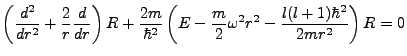$$\left(\frac{d^2}{dr^2} + \frac{2}{r}\frac{d}{dr}\right)R + \frac{... ...ar^2}\left(E - \frac{m}{2}\omega^2r^2 -\frac{l(l+1)\hbar^2}{2 mr^2}\right)R = 0$$ (3.12)

We can quickly solve this equation by applying the SAP method (Simplify, Asymptote, Power Series). We set the stage by first rewriting the above equation in a form which will later simplify our process,

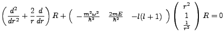$$\left(\frac{d^2}{dr^2} + \frac{2}{r}\frac{d}{dr}\right)R + \left(... ...ray}\right)\left(\begin{array}{c}r^2 \\ 1 \\ \frac{1}{r^2}\end{array}\right)R=0$$ (3.13)

Write $\mho^2 = \frac{m^2\omega^2}{\hbar^2}$, then our first asymptote is towards infinity where the $r^2$ terms dominate; our second is towards zero where $1/r^2$ dominates and we find that

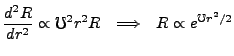$$\frac{d^2R}{dr^2} \propto \mho^2 r^2 R\ \ \Longrightarrow \ \ R \propto e^{\mho r^2/2}$$ (3.14)

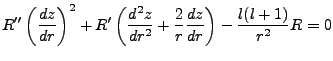
The next term is,

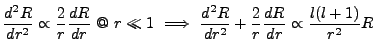$$\frac{d^2R}{dr^2} \propto \frac{2}{r}\frac{dR}{dr} \ @ \ r \ll 1 ... ...rrow \ \frac{d^2R}{dr^2} + \frac{2}{r}\frac{dR}{dr} \propto \frac{l(l+1)}{r^2}R$$ (3.15)

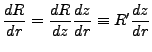
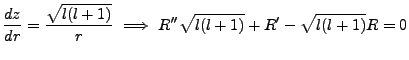
To solve such equations, we suppose there exist a function $z(r)$ which will bring this equation into a more conventionally solvable form. We will determine what z is by the consequences of this demand. With

$$\frac{dR}{dr} = \frac{dR}{dz}\frac{dz}{dr} \equiv R'\frac{dz}{dr}$$

$$\frac{d^2R}{dr^2} = R''\left(\frac{dz}{dr}\right)^2 + R'\left(\frac{d^2z}{dr^2}\right)$$

We now solve

$$R''\left(\frac{dz}{dr}\right)^2 + R'\left(\frac{d^2z}{dr^2} + \frac{2}{r}\frac{dz}{dr}\right)-\frac{l(l+1)}{r^2}R=0$$ (3.16)

This equation is solvable if the coefficients are proportional, or even better, equal:

$$\frac{dz}{dr} = \frac{\sqrt{l(l+1)}}{r} \ \Longrightarrow \ R'' \sqrt{l(l+1)} + R' - \sqrt{l(l+1)}R =0$$ (3.17)

This equation has solutions easily found as,

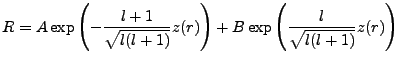$$R = A\exp\left(-\frac{l+1}{\sqrt{l(l+1)}}z(r)\right)+ B\exp\left(\frac{l}{\sqrt{l(l+1)}}z(r)\right)$$ (3.18)

But we can solve for z and find that 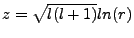$z=\sqrt{l(l+1)}ln(r)$, whereby,

$$R = Ar^{-(l+1)} + Br^{l}$$

We dismiss A since we are considering the infinitesimally near zero asymptote. Next we suppose our complete solution is a power series via,

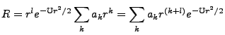$$R = r^le^{-\mho r^2/2}\sum_k a_k r^k =\sum_k a_k r^{(k+l)}e^{-\mho r^2/2}$$ (3.19)

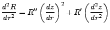
Our first derivative is,

$$\frac{dR}{dr} = \sum_k a_k\left((k+l)r^{k+l-1}e^{-\mho r^2/2} - \mho r^{k+l+1}e^{-\mho r^2/2}\right)$$

$$= \sum_k a_k r^{(k+l)}e^{-\mho r^2/2} \left(\begin{array}{cc}-\mho & k+l\end{array}\right) \left(\begin{array}{c}r\\ \frac{1}{r}\end{array}\right)$$

$$\frac{2}{r}\frac{dR}{dr} = \sum_k a_k r^{(k+l)}e^{-\mho r^2/2} \left(\begin{array}{cc}-2\mho & 2(k+l)\end{array}\right) \left(\begin{array}{c}1\\ r^{-2}\end{array}\right)$$ (3.20)

Our second derivative is,

$$\sum_ka_k\left((k+l)(k+l-1)r^{k+l-1}-\mho(2k+2l+1)r^{k+l}+\mho^2r^{k+l+2}\right)e^{-\mho r^2/2}$$

$$= \sum_k a_k r^{k+l}e^{-\mho r^2/2}\left(\begin{array}{ccc}\mho^2... ...l-1) \end{array}\right)\left(\begin{array}{c}r^2\\ 1\\ r^{-2}\end{array}\right)$$

Recalling that,

$$\left(\frac{d^2}{dr^2} + \frac{2}{r}\frac{d}{dr}\right)R + \left(... ...rray}\right)\left(\begin{array}{c}r^2 \\ 1 \\ \frac{1}{r^2}\end{array}\right)=0$$ (3.21)

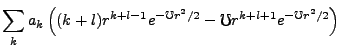
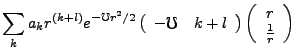
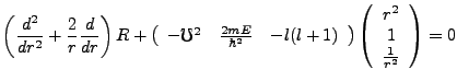
our net equation thus requires that

$$a_k r^{k+l}e^{-\mho r^2/2}\left(\begin{array}{cc}\frac{2mE}{\hbar... ...-l(l+1) \end{array}\right)\left(\begin{array}{c}1\\ r^{-2}\end{array}\right)=0$$

Or more simply,

$$r^{k+l}e^{-\mho r^2/2}\left(\begin{array}{cc}\frac{2mE}{\hbar^2}-... ...l+1)\end{array}\right)\left(\begin{array}{c}a_k\\ a_kr^{-2}\end{array}\right)=0$$ (3.22)

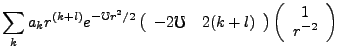
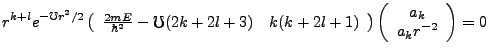
We seek to match the coefficients of r, since they must vanish independently, whereby,

$$r^{k+l}e^{-\mho r^2/2}\left(\begin{array}{cc}\frac{2mE}{\hbar^2}-... ...+2l+3)\end{array}\right)\left(\begin{array}{c}a_k\\ a_{k+2}\end{array}\right)=0$$ (3.23)

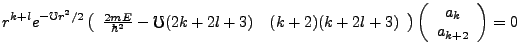
This gives us the recursion relation,

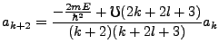$$a_{k+2}=\frac{-\frac{2mE}{\hbar^2}+\mho(2k+2l+3)}{(k+2)(k+2l+3)}a_k$$ (3.24)

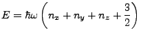
Requiring this series to terminate to prevent non-physical behavior is our quantization condition, whereby we must have,

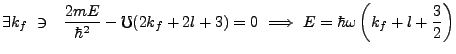$$\exists k_f \ \ni \ \ \frac{2mE}{\hbar^2}-\mho(2k_f+2l+3)=0 \ \Longrightarrow \ E = \hbar \omega \left(k_f + l + \frac{3}{2}\right)$$ (3.25)

This recursion relationship and eigenvalue formula thus define a three dimensional harmonic oscillator.