Space-Time Diagrams

We will begin with a basic introduction to space-time diagrams, which are very useful constructions in relativity theory. Nothing keeps your thinking clearer and cleaner than a good diagram, and that is especially true in SR when things are much more complicated to begin with.

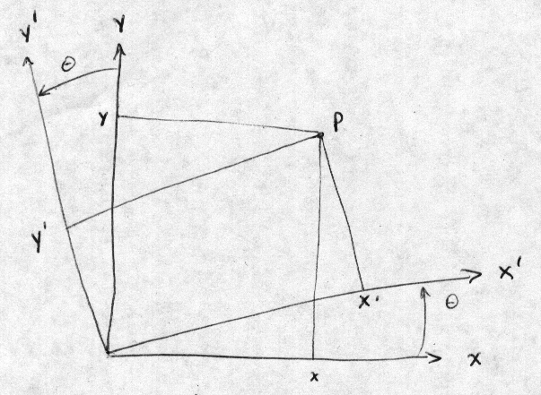
We'll build up our diagrams by first making an analogy. Consider two dimensional space. We can draw axis in the plane in different ways: say $x$ and $y$ ($S$ frame) or $x'$ and $y'$ ($S'$ frame) (see fig.1).

Figure 1: $xy$-plane with 2 different coordinate systems.

These two axis are related by a rotation by an angle $\theta$. If we do the appropriate geometry we see that the two are related by the following transformation:

$$\begin{eqnarray*} x' &=& x\cos(\theta)+y\sin(\theta)\\ y' &=& y\cos(\theta)-x\sin(\theta). \end{eqnarray*}$$

What these equations mean is that given any point $p$ in the plane with coordinates in $S$ given by $(x,y)$, we can find the corresponding coordinates of the same point in $S'$ given by $(x',y')$. Depending on our coordinate system, the same point can have different coordinates. We've known this since we started doing vector analysis: the same vector will have different components in different coordinate systems, but the length of the vector is the same in all of them.

In relativity, space and time are connected similarly to how the two dimensions of the plane were connected. If an observer is moving, her coordinate system is different, so she assigns different values of position and time to events than someone who is not moving.

Figure 2: Basic space-time diagram.

We can now draw a new diagram (fig.2) like the last one for this new situation. We begin by making our axis to be $x$ and $ct$, where $c$ is the speed of light (so that the time axis is measured as a length - the reason for this is forthcoming).

Note that we are accustomed to having time horizontal and space vertical when we draw graphs. But, space-time diagrams are always drawn the other way around. We just have to get used to this.

Now, any point on this graph is an event - it is a moment in space and in time. How about lines? If we let the slope of the line by measured from the $ct$-axis, its value will be

$$\tan(\theta)={\rm slope}=\frac{\rm opp}{\rm adj}=\frac{\Delta x}{c\Delta t} = \frac{v}{c}=\beta,$$

that is, the slope of the line is a speed. Thus we can interpret a straight line with slope $\beta$ from the $y-$axis as something moving with that constant speed. Moreover, the slope gives us the tangent of the angle made with the $y$ axis, $\beta=\tan\theta$.

What if it moves at the speed of light? Then the slope is $\beta=1$ and we have a line of slope $1$, that is, at $45^\circ$. This is why we scale the time axis by $c$ - to get the light rays to appear as $45^\circ$ lines. Light lines are of central importance in SR (they are invariants) so we want their representation to be as simple as possible. Note now that any physical motion must have $\beta<1$, so that the line representing that motion is always sloped less with respect to the $y$-axis than $45^\circ$.

Now, since a sloped line represents the motion of another observer, say, that's the next part of the diagram. That line is the time axis $ct'$ of the moving observer. What about the $x'$ axis? Well, remember that Lorentz transformations preserve the speed of light, so we must have

$$c=\frac{\Delta x}{\Delta t}=\frac{\Delta x'}{\Delta t'},$$

which means that if the $t'$ axis is rotated to the right by $\theta$, then the $x'$ axis is rotated up by $\theta$! (See fig.3).

Figure 3: Space-time diagram with two reference systems.

Now we can represent two (or more) observers on the same graph. We answer all of our questions by translating between coordinates in $S$ and coordinates in $S'$ by using the Lorentz transformation equations:

$$\begin{eqnarray*} x' &=& \gamma (x-\beta ct)\\ ct' &=&\gamma (ct-\beta x). \end{eqnarray*}$$

What we have done so far is build a little machinery to make SR calculations easier. Learning new machinery is difficult for 2 reasons. First, it's something new to learn and we might now know how to apply it. Second, we don't know how this will actually make our lives easier - it's just excess baggage. Well, we'll use these diagrams to solve most of the problems in this chapter and through these examples we'll gain an appreciation of how these help clarify the problems at hand.