Software registered with the Python Package Index (PyPI).
Available in a git repository.
Repository: h5config
Author: W. Trevor King
Since the number of packages mooching off pypiezo's configuration scheme was growing, I've split it out into it's own package. Now there's a general package for all your HDF5-based configuration needs.
The README is posted on the PyPI page.
Available in a git repository.
Repository: pypid
Author: W. Trevor King
I've just finished rewriting my PID temperature control package in pure-Python, and it's now clean enough to go up on PyPI. Features:
- Backend-agnostic architecture. I've written a first-order process with dead time (FOPDT) test backend and a pymodbus-based backend for our Melcor MTCA controller, but it should be easy to plug in your own custom backend.
- The general PID controller will automatically tune your backend using any of a variety of tuning rules.
The README is posted on the PyPI page.
Available in a git repository.
Repository: insider
Author: W. Trevor King
Insider is a little Django app I wrote to help my brother, Garrett, track insider trading with a simple, familiar web interface. It's a pretty simple app, partly thanks to Bradley Ayers' django-tables2, which does the table formatting. Just goes to show that a good scripting language and framework make developing simple apps a breeze!
The README is posted on the PyPI page.
Available in a git repository.
Repository: pypiezo
Author: W. Trevor King
This is a piezo-actuator control library based on pycomedi. It also contains some atomic-force-microscope-specific logic. The higher-level library pyafm extends the AFM-control framework with coarse positioning.
The README is posted on the PyPI page.
Available in a git repository.
Repository: calibcant
Author: W. Trevor King
Here is my Python module for AFM cantilever calibration via the thermal tune method.
The README is posted on the PyPI page, and you might also be
interested in the package dependency graph generated
with Yu-Jie Lin's PDepGraph.py:
# python PDepGraph.py -o calibcant.dot \
    -D matplotlib,scipy,numpy,pyyaml,h5py,python,eselect-python \
    calibcant
# dot -T svg -o calibcant.svg calibcant.dot
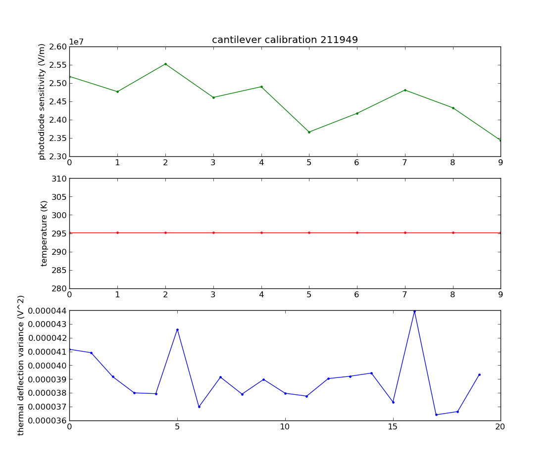
Thermal calibration requires three separate measurements: photodiode sensitivity (via surface bumps), fluid temperature (estimated, or via thermocouple), and thermal vibration (watching the cantilever vibrate in far from the surface). The calibcant package takes repeated measurements (statistics.png) of each of these parameters to allow estimation of statistical uncertainty:
# calibcant-analyze.py calibcant/examples/calibration.h5
...
... variable (units)         : mean +/- std. dev. (relative error)
... cantilever k (N/m)       : 0.0629167 +/- 0.00439057 (0.0697838)
... photo sensitivity (V/m)  : 2.4535e+07 +/- 616119 (0.0251118)
... T (K)                    : 295.15 +/- 0 (0)
... vibration variance (V^2) : 3.89882e-05 +/- 1.88897e-06 (0.0484497)
...
While this cannot account for systematic errors, calibration numbers are fairly meaninless without at least statistical error estimates.
Extracting the photodiode sensitivity and thermal deflection variance from the raw data can vary a suprising amount depending on your cantilever/photodiode linearity and drift and signal/noise ratio in the vibration data. To help deal with this, calibcant provides a choice of models for fitting each measurement type.
The contact region of surface bumps can be fit with either linear or quadratic models. Here is an example of a single surface bump fit with a quadratic model. The green line is the initial guess (before fitting), the red line is the final model (after fitting), and the blue dots are measured data points. The red dots in the bottom panel are the residual, which looks cubic because we've subtracted a quadratic model.

Extracting the thermal vibration variance is also trickier than it might seem. Fitting the data in frequency-space to a Lorentzian (Breit-Wigner?) model helps filter out low frequency drift, as well as white noise from the measurement equipment.
where and come from the damped-forced harmonic oscillator equation of motion
the cantilever's effective mass is , and is an optional white-noise offset.
Here is an example of a one-second thermal vibration fit with the offset Breit-Wigner model. The top panel is the time-series deflection voltage (bits vs sample index). The center pannel is a histogram of the deflection voltage, showing an approximately Gaussian distribution. The bottom panel shows the power spectral density fit (red dots) fit with an offset Breit-Wigner model (blue curve). The horizontal blue line marks the white-noise offset, and the vertical blue line marks the resonant frequency. Points outside the light blue region were not considered during the fitting. This allows us to isolate the cantilever's thermal vibration from other noise sources, which leads to more accurate and reproducible spring constant estimates.

Finally, all data and analysis results are stored in the standard, portable HDF5 file format, so it's easy to reanalyze earlier calibration data with different models if you decide to do so at a later date, or just look back and see exactly what calculations went into your spring constant calibration in the first place.
I tried to build calibcant on top of a chain of packages to make swapping out the hardware interface easier, but Comedi is at the bottom of the current chain, so it may be hard to use this package if you're not running Linux. If you're not running Linux, but are interested in getting calibcant working on your system anyway, send me an email! I'd be happy to help generalize calibcant, but it's hard for me to imagine hardware control from Windows (do people run experiments from Macs?). If you've figured that part out, I can probably graft calibcant onto your system.
Available in a git repository.
Repository: FFT-tools
Author: W. Trevor King
AFM cantilever calibration via thermal tuning requires unitary Fourier transforms, but Numpy's DFT is not unitary. This module provides some simple unitary wrappers with an associated test suite.
The README is posted on the PyPI page.