Our cantilever can be approximated as a damped harmonic oscillator
In the following analysis, we use the unitary, angular frequency Fourier transform normalization
 |
(29) |
We also use the following theorems (proved elsewhere):
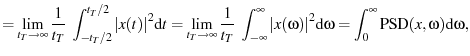
We also use the Wiener-Khinchin theorem,
which relates the two sided power spectral density
![]() to the autocorrelation function
to the autocorrelation function ![]() via
via
| [15] | (36) |
For highly damped systems, the inertial term becomes insignificant
(
![]() ).
This model is commonly used for optically trapped beads. Because it is simpler and solutions are more easily available,
we'll use it outline the general approach before diving into the general case.
).
This model is commonly used for optically trapped beads. Because it is simpler and solutions are more easily available,
we'll use it outline the general approach before diving into the general case.
Fourier transforming eq. 28 with ![]() and applying 31 we have
and applying 31 we have
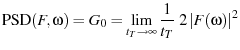
Because thermal noise is white (not autocorrelated + Wiener-Khinchin Theorem), we can denote the one sided thermal power spectral density per unit time by
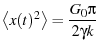
Plugging eq. 40 into 39 we have
 |
(41) |
Integrating over positive ![]() to find the total power per unit time yields
to find the total power per unit time yields
 |
(42) | |
 |
(43) | |
 |
(44) |
Plugging into our corollary to Parseval's theorem (eq. 34),
Plugging eq. 45 into eqn. 1 we have
| (46) | ||
 |
(47) |
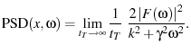
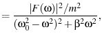
So we expect ![]() to have a power spectral density per unit time given by
to have a power spectral density per unit time given by
 |
(48) |
The procedure here is exactly the same as the previous section.
The integral normalizing ![]() just become a little more complicated...
just become a little more complicated...
Fourier transforming eq. 28 and applying 31 we have
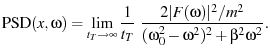
We compute the
![]() by plugging eq. 51 into 33
by plugging eq. 51 into 33
Plugging eq. 40 into 52 we have
 |
(54) | |
 |
(55) | |
 |
(56) | |
 |
(57) | |
 |
(58) |
Plugging eq. 59 into the equipartition theorem (eqn. 1) we have
 |
(60) | |
 |
(61) |
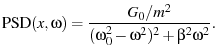
So we expect ![]() to have a power spectral density per unit time given by
to have a power spectral density per unit time given by
![$\displaystyle \ensuremath{\operatorname{PSD}}(x, \omega) = \frac{2 k_BT \beta} {\pi m \left[ (\omega_0^2-\omega^2)^2 + \beta^2\omega^2 \right] }$](img125.png) |
(62) |

![$\displaystyle = \pm\sqrt{\frac{1}{2}[1+\cos(\theta)]}$](img74.png)