Next: 3 Theoretical power spectral
Up: cantilever_calib
Previous: 1 Overview
Subsections
To find  , the raw photodiode voltages
  are
converted to distances
are
converted to distances  using the photodiode sensitivity
 (the slope of the voltage vs. distance curve of data taken
while the tip is in contact with the surface) via
(the slope of the voltage vs. distance curve of data taken
while the tip is in contact with the surface) via
 |
(5) |
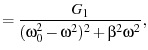
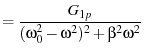
Rather than computing the variance of directly, we attempt to
filter out noise by fitting the spectral power density (
 ) of
to the theoretically predicted
for a damped harmonic
oscillator (eq. 53)
) of
to the theoretically predicted
for a damped harmonic
oscillator (eq. 53)
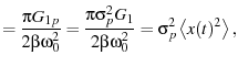
where
 ,
,  , and
, and  are used as the
fitting parameters (see eqn.s 53). The variance of
is then given by eq. 59
are used as the
fitting parameters (see eqn.s 53). The variance of
is then given by eq. 59
 |
(8) |
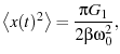
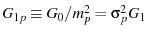
which we can plug into the equipartition theorem
(eqn. 1) yielding
 |
(9) |
From eqn. 61, we find the expected value of  to be
to be
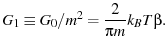 |
(10) |
In order to keep our errors in measuring seperate from
other errors in measuring
 , we can fit the voltage
spectrum before converting to distance.
, we can fit the voltage
spectrum before converting to distance.
 |
 thermal thermal |
(11) |
 |
 |
(12) |
|
 |
(13) |
 |
 |
(14) |
 |
 |
(15) |
where
 ,
,
 .
Plugging into the equipartition theorem yeilds
.
Plugging into the equipartition theorem yeilds
 |
 |
(16) |
From eqn. 10, we find the expected value of  to be
to be
 |
(17) |
Note: the math in this section depends on some definitions from
section 3.
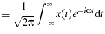
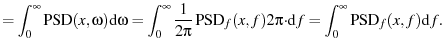
As yet another alternative, you could fit in frequency
 instead of angular frequency
  . But we
must be careful with normalization. Comparing the angular frequency
and normal frequency unitary Fourier transforms
. But we
must be careful with normalization. Comparing the angular frequency
and normal frequency unitary Fourier transforms
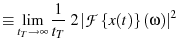
from which we can translate the
The variance of the function is then given by plugging into
eqn. 34 (our corollary to Parseval's theorem)
 |
 |
(22) |
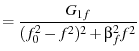
Therefore
where
 ,
,
 , and
, and
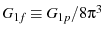 . Finally
|
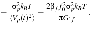 |
(26) |
From eqn. 10, we expect  to be
to be
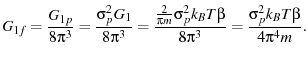 |
(27) |
Next: 3 Theoretical power spectral
Up: cantilever_calib
Previous: 1 Overview
Download cantilever_calib.pdf
View the source files or my
.latex2html-init configuration file
2 Methods
Copyright © 2009-10-12, W. Trevor King
(contact)
Released under the GNU Free Document License, Version 1.2 or later
Drexel Physics