Programming Strategies
 Back to course contents
An ideal program running on a parallel computer ought to be
perfectly scalable, i.e., increasing the number of processors
by a multiplicative factor N should
decrease the time spent to
perform the task by
a factor 1/N.
However, in practice, very few programs achieve this level of
scalability. There are three major causes for this:
- Existence of sequential parts in the algorithm
- Necessity of node to node communications
- Load unbalance
This leads to the following rules in order to obtain
high performance on a parallel computer:
Rule #1: Adapt the algorithm to the parallel platform
Adapting a sequential code to run on a parallel computer often
requires some major changes in the algorithm in
order to obtain good performance. A major guiding
principle is to maximize the
work done simultaneously on the different nodes. An
important issue here is data dependency;
for instance, if node 0 requires x after node
1 has calculated x, then it will have to wait
until node 1 releases x before proceeding with
x. This situation can lead to undesirable
bottlenecks in the computation since synchronization
among nodes then becomes necessary. This is never an issue for
sequential codes.
Data dependency may lead to race conditions, and possibly
wrong answers, in addition to slowing down the process.
A race condition occurs when the answer of a series of operations
depends on the order in which the operations are performed.
As an
example, if x=0 and x=1 should be executed on different nodes,
you have to make sure the order of execution is in the right order to
get the answer correctly; this implies synchronization.
A second major issue is granularity. Should you divide the
problem in very many tiny parcels (fine graining),
or should you divide the problem solution in big chunks
(coarse graining). The physical problem
often dictates the answer here.
Even the best algorithms will often
harbor some sections which are intrinsically sequential.
This fact is expressed in Amdhal's law, which says that
a program can only be sped up by the use of a parallel
computer in the sections of the algorithm which is
parallelized. The solution is often here to re-think
the algorithm to minimize the serial sections.
Rule #2: minimization of node to node communication
Node to node communication in a distributed memory parallel
computer is orders of magnitude slower than direct fetching
of variables from local memory. Much node to node communication
will invariably result in node idle time and therefore performance
degradation. Communication should be minimized, leading to an
enhanced ratio computation/communication.
The ideal parallel application is
one in which all nodes would compute totally independently
from each other with no need for any communication. As examples
of such applications,
the analysis of the different events in a high-energy experiment
are independent from each other; also the analysis of
chaotic scattering
falls in this category. These
problems typically only have a small quantity of results to
gather at the end of each task on the different nodes.
These types of problems are often labeled as "trivially
parallizable".
On the other hand, some problems intrinsically
require much node to node communication. Solving
Partial Differential Equations (PDEs) often falls
in this category. We will be more explicit about
this case when we address
domain decomposition.
Latency is a determining factor in communication. If many
small messages are to be transmitted, it might be more efficient to
group these into a large message.
Rule #3: Load balancing
Scalability in a parallel application can only be obtained
if all the nodes are given tasks requiring the same amount
of time to perform.
This seemingly trivial statement is of great importance
in guiding the writing of parallel applications. It says
that you must organize the flow of operations in such
a way that the nodes idle the least possible amount.
Interestingly enough, the problems that were characterized as
trivial parallel applications from the point of view of
communications are not so from the point of view of load
balancing. A regular scattering trajectory
is likely to take much less
time to calculate than a chaotic one! This may lead to load
unbalance if one is not careful. The solution of PDEs
by domain decomposition on the other hand will often naturally
yield load balancing.
Solutions to this load balancing problem can often be
found in a careful
re-write of the algorithm so as to distribute the load more
evenly among the nodes. There are two approaches:
- Static Load Balance
- Dynamic Load Balance
 Back to top of page
In static load balance the programmer assigns a pre-determined
amount of work to each processor.
This solution often only
requires a re-ordering of the calculation as done in a sequential
machine and so is often easier to
implement than any other solution. This approach
can be implemented on hostless
computer, in which all the nodes are equivalent. This is often the approach used
in the bulk of codes solving partial differential equations.
Back to top of page
The dynamical load balancing approach
requires the Master-Slave model.
In this model, a node, the so-called master node,
administers the work to be done by all other slave nodes.
The distribution of tasks among the nodes is illustrated
in the following flowchart.
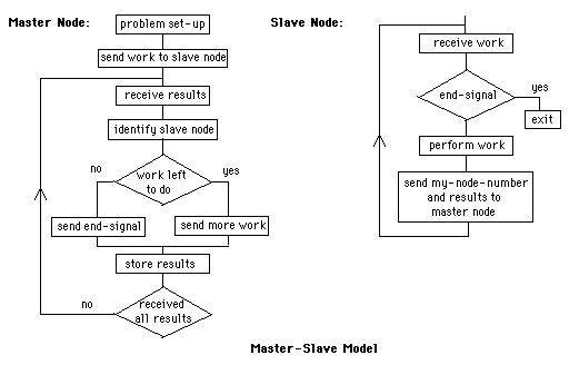
As soon as a slave node finishes its work, it sends the
results back to node 0; this triggers node 0 to send it
more work to do. As long as the global task is parceled
into sufficiently small segments, this should produce
very small amount of idle time in the various slave nodes.
Of course, the master node is not kept very busy in this model.
This paradigm applies better to an inhomogeneous system, whereby
the master node could be the front-end computer
of a parallel machine, typically a slow computer itself.
We will illustrate the master-slave model using node 0
as the master node. To do so, we will use the Mandelbrot Set
as an example. We will describe how one can go from a sequential
code to a parallel code in so doing.
Back to top of page
Mandelbrot discovered the set bearing his name in 1980. It is
considered today as one of the most complicated objects mathematics
has ever considered. It produces incredibly beautiful and complicated
pictures. You can find fascinating renditions of the set by exploring
the Web; look in particular at the wikipedia site:
http://en.wikipedia.org/wiki/Mandelbrot_set
The Mandelbrot Set (M) results from a very
simple map in the complex plane:
	z    =   z  z   + c
	 i+1      i  i
by following the following rules:
- for a given complex number c,
start with z = 0, and iterate the map above
- if z remains finite, even after an infinite number
of iterations, c belongs to M
- repeat the procedure, or scan, for all c
in the complex plane, to find
the points belonging to M!
The code mandelbrot.c
generates the Mandelbrot Set via a direct coding of the
rules given above. This leads to a somewhat slow algorithm to generate
the Mandelbrot Set; so be it! We only need to
use this code as an example as how to implement a
parallel version of the code.
An excellent way to display a function
of two variables, f(x,y), is to form
a color image whereby the color of each
pixel corresponds to the value of f(x,y)
at that location. The tool to accomplish
this must translate the function range
to a color palette range. For our
purpose, this tool must read in a
2-dimensional array containing the values
of f(x,y) on a 2-dimensional lattice
and produce the color image.
The python script
plot_image.py
does precisely this. It is based
on the matplotlib.
matplotlib
is a Python 2-dimension plotting library which
produces publication quality figures with
great flexibility in a variety of formats.
The web site
matplotlib.sourceforge.net
describes how to download, install and use
this library. The tutorials, user's guide
and examples found in this site are easier to read
by a reader with some previous knowledge of
Python and Numerical Python.
Use
gen_data.c,
gen_data_sharp.c and
gen_data_rectangle.c
to form simple images by feeding sample data in plot_image.py.
These codes produce
images of size ($N_x = 200 \times N_y = 200$ )
and ($N_x = 300 \times N_y = 200$ )
for the third code respectively.
Read the comments
in plot_image.py to learn how to use it.
Practice the different options.
can also display color rendition of data
sets in 2-dimensions. An easy way to accomplish this is
via the matrix notation.
As an example, let us display the Mandelbrot Set. The steps
could be
This gnuplot option requires the data
to be written such that each row of the matrix is written
on a (one) separate line, each matrix element being separated by a blank
from the adjacent elements.
We will parcel the task of computing the Mandelbrot Set
by slicing the complex plane into vertical stripes,
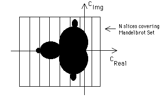
and asking each of the slave nodes to find the points
within each strip belonging to the Mandelbrot Set. In fact we will
write the code for horizontal (parallel to C_img) stripes.
The stripes in the middle of the Mandelbrot set
take long time to compute, while those practically outside
of the set are fast to compute. The master-slave model accommodates this fact by
having the master code ready to supply a new stripe to compute as soon as a
slave ends its task of computing a current slice.
The adaptation of a code to run in parallel most of the time requires new
algorithms or at
least a deep rewrite of the serial code. This is often the case that the
flow of the calculation needs profound modification.
The code for generation of the Mandelbrot Set is no exception.
In this case
we need to accomodate the slicing of the domain in C.
Much of the rewrite can often be
done in a new version of the the serial code.
As a first step, we rewrite the
mandelbrot.c code to
make it more modular. Since the parallelization of the code will imply
a new main()
code, one should simplify the main routine via function calls to make
the overall logic as clear as
possible; call this new version MS1.c. Write two new functions: set_grid()
which sets the grid up and iterate_map() which iterates the Mandelbrot Map. These
functions must have appropriate arguments. This code should produce the same results
as the previous one.
This code is listed in
MS1.c
Next we must
take into account the slicing of the complex plane. Modified the code into a new serial
code called MS2.c. Introduce two new functions (careful with the arguments)
called set_slices() and calculate_slice() with the obvious
functionality based on their names.
A loop
for ( slice=0 ; slice < N_slices ; slice++ )
in the main program will then do the trick.
You might specify 64 slices in the code as an example.
This code should produce the same results
as the previous one.
This code is listed in
MS2.c
The parallel implementation is now relatively simple.
You should write yet two new functions,
master() and slave() (with appropriate arguments)
that implement the logic illustrated in the flowcharts above.
The steps to follow are (you may want to save a version for each major steps below):
- Version #1 (global code logic)
- Introduce MPI variables & MPI administration routines (MPI_Init(),
MPI_Comm_size(), MPI_Com_rank()
- Add calls to master() and slave() in the main code
- set slave() to receive a slice # and compute the
Mandelbrot set in the requested slice
- set an initial slice distribution to slave processes
- set sent_stripe & recv_stripe logic in master()
- use fprintf( stderr, ...) diagnostic print statements if need be
- Version #2 (basic results send/receive logic)
- send result back in slave processes
- set receive structure in master process
- Version #3 (slave termination logic)
- set slave termination logic
- send termination signal from master process
- Version #4 (work flow logic)
- set the not-yet-done slices logic
- send new slice to appropriate slave process (modification of stripe
sending logic in Version #1)
- Version #5 - Final version (output results)
- remove all output from original code
- pack slice results in a large array
- output array
Each of the versions above can be run on the parallel machine. Some might
hang the machine, yet allow the debugging to be done. <CTRL>-c allows to
break an MPI run. The final parallel code, call it MS3.c,
should produce the same image as the original serial code.
This code is listed in
MS3.c
Back to top of page
Back to course contents