Monte Carlo Techniques

Back to course contents

Monte Carlo Integral
Calculation of π
Applicability of the Method
Metropolis Algorithm
Guided Monte Carlo Integral
Parallel Monte Carlo Algorithm
Random Numbers Generation
Parallel Monte Carlo Codes

The Monte Carlo technique to perform integrals applies best to higher dimensional integrals for which other traditional methods become difficult. For instance, using few hundred points to perform a 1-D integral using the trapezoidal or Simpson method is easily done. However, the same in multi-dimension does not apply: a five dimensional integral

$I = \int dx_1 \int dx_2 \int dx_3 \int dx_4 \int dx_5 f( x_1, x_3, x_3, x_4, x_5 )$
would require 200⁵ function evaluations to implement a method with 200 points per axis. Statistical Physics requires integrals of much higher dimensions, often of the order of the number of particles.

The Monte Carlo approach deals with this problem by sampling the integrand via statistical means. The method calls for a random walk, or a guided random walk, in phase space during which the integrand is evaluated at each step and averaged over.

This problem is presented here as a challenging case to implement via a parallel algorithm. Different implementations will require us to use all the MPI functions we have seen so far. In the following, the Monte Carlo method will first be explained, then it will be implemented serially, and then the Metropolis algorithm will be explained, and implemented serially and in parallel.

Back to top of page

Monte Carlo Integral

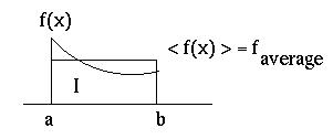
The Monte Carlo Method is best explained via a 1-D integral

$I = \int_a^b f(x) dx$
Rewrite

I = (b-a) < f(x) >

where <f(x)> is the average of f(x) over the interval (a,b).

$< f(x) > = \frac{1}{N} \sum_{i=1}^{N} f(x_i)$

The Monte Carlo method consists in choosing the sampling points x_i at random in the interval (a,b).

The advantage over other methods in higher dimension is that better coverage of the function can be achieved with fewer points in phase space.

The error in evaluating <f> is described by the variance

$\sigma^2 = \frac{1}{N} \left[ < f^2 > - < f >^2 \right]$

Back to top of page

Calculation of π

The method is illustrated by integrating f(x,y)=1 in a circle, namely

$I = \int_{-1}^{1} dx \int_{-1}^{1} dy \Theta( 1 - x^2 -y^2 )$
This corresponds to

$I =\int_{-1}^{1} dx \int_{-1}^{1} dy \left[ \begin{array}{ll} 1 & if x^2+y^2 \leq 1 \\ 0 & if x^2+y^2 > 1 \end{array} \right.$
The Monte Carlo approach is implemented by enclosing the circle in a square of side 2 and using random numbers in the interval x = (-1,1) and y = (-1,1). The area of the circle is π 1² and the area of the square is 2². The ratio of these areas is then π/4.

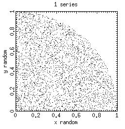
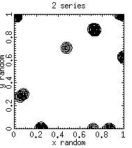
Random numbers, taken as x - y coordinates of points in a plane evidently fill in the plane uniformly. Therefore, the numbers of random numbers that fall within the circle and the square are proportional to their areas. Therefore

π = 4 # hits in circle / # random numbers

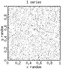
The program random_demo.c generates x and y coordinates in the interval (0,1) via calls to RAND( ), the build-in pseudo random-number generator function in the "C" compiler. The code is serial and can run on any computer.

random_demo 2000 > data_file

runs the random_demo to produce 2000 random points which are piped in a file data_file. The latter can be plotted using gnuplot. It produces the following graph.

The program monte_pi_serial.c calculates π by the Monte-Carlo method. It uses random numbers in the interval [0,1].

The error in calculating π follows from the standard deviation calculation in the following way:

$\sigma^2 = \frac{1}{N} [ < f^2 > - < f >^2 ]$
$\sigma^2 = \frac{1}{N} \left[ \frac{1}{N} \sum_{i=1}^{N} 1 - ( \frac{1}{N} \sum_{i=1}^{N} 1 )^2 \right]$
$\pi = \frac{1}{N} \sum_{i=1}^{N} 1$
$\sigma^2 = \frac{\pi}{N} \left( 1 - \pi \right)$

Back to top of page

Applicability of the Method

The random sampling of a function clearly works best if the function is a constant. (Why don't you then get the exact value of π in the example above?) If the function varies rapidly, or is locally peaked, the Monte Carlo method will not converge as rapidly. What is required is a "guidance" of the random sampling that emphasizes sampling where the function is large or varies rapidly. Let's illustrate the concept in 1-D.

$I = \int_0^1 f(x) dx$
Introduce a weight function w(x)

$I = \int_0^1 w(x) \frac{f(x)}{w(x)} dx$
where w(x) is required to satisfy

$\int_0^1 w(x) dx = 1$
Change variable to y

$y(x) = \int_0^{x'} w(x') dx'$
such that

dy = w(x) dx, y(0) = 0, and y(1) = 1.

$I = \int_0^1 dy \frac{ f( x(y) ) } { w( x(y) }$
The weight function w(x) is chosen such that [f/w] is aproproximately constant. The Monte Carlo sampling of [f/w] with uniform random sampling in y variable will then be accurate.

$I = \frac{1}{N} \sum_{i=1}^{N} \frac{ f( x(y_i) ) } { w( x(y_i) }$
Koonin and Meridith (Computational Physics, 1989) give the example

$I = \int_0^1 dx \frac{1}{1+x^2}$
with

$w(x) = \frac{1}{3} ( 4 - 2 x )$
In this simple case, the inversion x(y) is possible analytically.

$y = \frac{1}{3} x ( 4 - x )$
x = 2 - (4 -3 y )

In general, this inversion x(y) is difficult or impossible to perform analytically. An alternate approach must be used.

The relation dy = w(x) dx implies another interpretation of the method. Random numbers uniformly distributed in y will be distributed according to w(x) in x. Therefore, the guiding action of w(x) can be achieved by generating random numbers according the the probability profile w(x). This holds in phase spaces of arbitrary dimension. The problem translates into that of finding random distribution of arbitrary probability distributions.

Uniform random numbers in interval (0,1) have an average value of 0.5. A binning in intervals dx will show an average number of random number

number / bin = total # of random numbers / number of bins.

The number of random numbers in the bins will fluctuate around the average with a Gaussian distribution.

Random numbers distributed according to the distribution w(x) will bin according to w(x).

Back to top of page

Metropolis Algorithm

The Metropolis algorithm generates a random walk guided by the weight function w(x). The algorithm in 2-D involves the following steps. Starting from a point (x_i, y_i).

choose η (step size)
generate 2 uniformly distributed random numbers, R₁ and R₂, in the interval (-1,1)
calculate a new trial point according to
$x_{i+1}^T = x_i + \delta x_R$
$y_{i+1}^T = y_i + \delta y_R$
where the steps in x and y are η R₁ and η R₂ respectively
evaluate the ratio of the weight function at the trial point to the one at the old point
$r = \frac{ w( x_{i+1}^T, y_{i+1}^T ) } { w( x_{i}, y_{i} ) }$
if r>1, accept the new point (x_i+1,y_i+1) = (x_i+1^t,y_i+1^t) and loop back to step (2)
if r<1, accept the new point with probability r. That is, generate R, a random number in the interval (0,1), and accept (x_i+1^t,y_i+1^t) as the new point (x_i+1,y_i+1) if r > R and loop back to step (2)
otherwise, reject it, and keep the previous point as the new one (x_i+1,y_i+1) = (x_i,y_i)
loop back to step (2)

Koonin and Mederith (Computational Physics, 1989) provide a simple proof that the algorithm produces the desired random number distribution w(x).

The step η in the Metropolis algorithm is arbitrary. If chosen small, the acceptance ratio will be high (a point in the neighborhood of an acceptable point will also likely be acceptable). But overall coverage of the phase space will be very slow. If η is large, the phase space will be efficiently covered, but a new point will seldom be accepted by the Metropolis criteria. In either case ineficiency follows. An empirical rule is to choose η such as to have an acceptance ratio about 0.5 - 0.6.

A concern about the algorithm is that the random numbers generated by the Metropolis algorithm are correlated. A way to guard against this (Koonin and Mederith , Computational Physics, 1989) is to calculate the correlation functions

$c(k) = \frac{ <f_if_{i+k}> - <f_i>^2 } { <f_i^2> - <f_i>^2 }$
and select each k^th random number generated by the algorithm with k selected to produce a small value of C_k.

Back to top of page

Guided Monte Carlo Integral

Lets consider the integral
$I = \int dx \int dy (x^2+y^2) e^{ - (x^2+y^2) }$
The integral is peaked (torus shape) around the origin.

The Gaussian function

$w(x,y) = \frac{1}{\pi} e^{ - (x^2+y^2) }$
can be chosen to guide the random number selection.

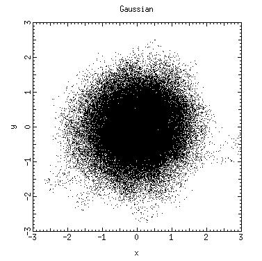
The program Metropolis_Gaussian_Demo.c illustrates a random numbers generation according to w(x,y). Note that arbitrary values for the step size (η=0.2) and k (k=1) were chosen; no effort was made to chose them optimally.

This code, with 2000 points, produced the following random number distribution.

The program Metropolis_Gaussian_Integral.c performs the integral.

Metropolis_Gaussian_Integral -p > data_file
or
Metropolis_Gaussian_Integral

This code prompts the user for more points to be added to the Monte Carlo integral. The calculation of the error may show the calculation not to be accurate given that the choices of η and k were not optimized.

Back to top of page

Parallel Monte Carlo Algorithm

Random Numbers Generation

Pseudo random numbers are often generated by a linear congruent algorithm. The integer random number x_i+1 is generated from the previous one by
x_i+1 = ( x_i a + b ) _{mod c}
The coefficients a, b and c are chosen to generate statistically good random numbers in a specific integer range (Numerical Recipes). Often the random numbers are generated using different linear congruence relation, and mixed via random selection as in RAND1 and RAND2 (Numerical Recipes).

The procedure to generate random numbers is deterministic. Two different nodes on a parallel machine will produce exactly the same sequence if "seeded" in the same way. The question then arises as to how to generate "good" random numbers on the different nodes of the parallel computer that will remain meaningful when used as a single set.

One solution is to generate sequences on each node based on different seeds. The code random.demo_2_series.c simulates this approach by generating 1 or 2 sequences of random numbers that can be analyzed for their goodness. The idea is to look for the goodness of a sequence in which the first and second half of the series are generated with different seed versus sequences generated from a single seed.

random_demo_2_series 2 1000 > data_file

The following filters can be used to acquire some feelings for the goodness of these random numbers

void.c which locates voids in the plane covered by 1 or 2 sequences of random numbers. This can be used to illustrate differences in coverage of the plane in short sequences. Example:
random_demo_2_series 2 1000 | void > data_file
produces the following graphs in gnuplot for 1 and 2 seeded series of 1000 points
bin_distribution.c which bins the random numbers in a 2-D grid, then further bins the distribution as a function of the number of random numbers per bin.
random_demo_2_series 2 20000 | bin_distribution > data_file
produces the following distributions for large sequences of random numbers

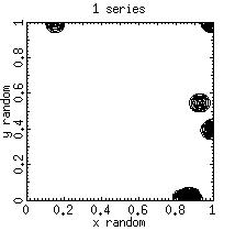
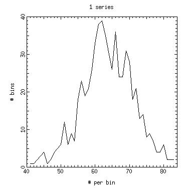
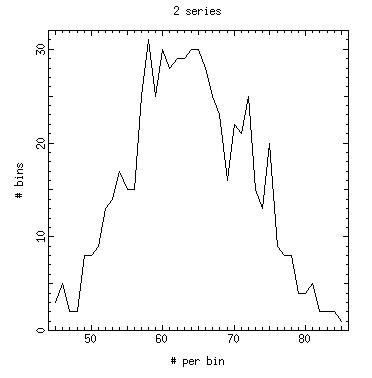
Clearly the random numbers sequences generated from sequences using different seeds have different properties than sequences generated from single seed.

We use here the approach that Random numbers should be generated on one node and distributed to the nodes which need them. This avoids the use of sequences generated from different seeds. Realistic applications often require time-consuming function evaluations. Therefore the inefficiency inherent in our approach is dwarfed by the large function evaluation times. This is also the approach used by Gropp et al. in "Using MPI".

Back to top of page

Parallel Monte Carlo Codes

A parallel implementation of the Monte Carlo integration must have the random sequence distributed to the different nodes, either by communication or by a local generation of the sequence. We implement here three versions of the code.

Master-Workers paradigms

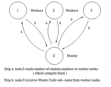
This code generates the random numbers on nodes 0 and passes them onto the worker nodes. The latter compute the Monte Carlo sub-sums and pass these sub-sums to node 0 which finishes the sums. The MPI_Reduce() function can be used to expedite the global sums

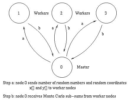
Metropolis_Gaussian_Parallel.c implements this approach.

Client-Server paradigm

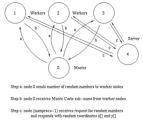
This code implements the concept of a random number server; this is a node reserved to serve random numbers with weight w(x,y) to whichever node requests it. The code sets node 0 as a master node to direct the calculation and interface with the user. Node (numprocs-1) is the random numbers server, and nodes 1 to (numprocs-2) are the worker nodes which complete the Monte Carlo sub-sums.

The code Metropolis_CS.c implements a version of of this approach in which the functionality of the different nodes is relegated to C functions. This illustrates the fact that variables are local to the nodes.

Gropp et al, in "Using MPI" implements this version of a Monte Carlo integration to calculate π.

Full Workers version

In this version, node 0 administers the ranges of random numbers to be generated for each workers, but leaves the actual generation of the random numbers to the nodes themselves. Upon receiving a range, i.e., random numbers range 1001 to 2000, the worker nodes generate these numbers and calculate the Monte Carlo sub-sums. This implies that they must generate and discard those random numbers prior to their range selection. This is a waste of computing cycles, but given the speed of computing versus the network speed it maybe the most efficient approach after all.

The scheme is therefore

It is left to the reader to implement this approach.

Back to top of page

Back to course contents