• Parabolic Equation
• Model
• Parabolic PDEs solution
• Serial Implementation

Parabolic Equation

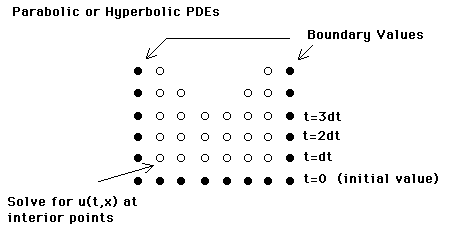
PDEs are traditionally classified into three broad categories: elliptic, parabolic and hyperbolic equations. However, from the numerics point of view, PDEs divide into static equations (elliptic) and time dependent equations (parabolic & hyperbolic).

The hyperbolic and parabolic equations represent initial value problems. The diffusion equation (parabolic)

(D is the diffusion coefficient) is such that we ask for what is the value of the field (wave) at a later time t knowing the field at an initial time t=0 and subject to some specific boundary conditions at all times.

The domain may be 1-D, 2-D, or 3-D. This equation might represent a heat diffusion problem in which the temperature within the domain is sought at all times, starting from a given temperature field at the initial time, and preserving the temperature at the boundary of the domain. In addition, a source term S(x,t) could be added to the right hand side of the equation. If u(x,t) represents a temperature field, then S(x,t) would represent a heat source.

The parallelization of the solution of a PDE of parabolic or hyperbolic PDEs is obtained through domain decomposition. However, in this case, the Domain Decomposition applies only to the space variables. The time evolution is essentially sequential, is obtained from , which can not be parallelized. 

Model

We will model heat diffusion through a 2-D plate.    The parabolic PDE to solve is 

∂ u(x,y,t) / ∂ t = ∂² u(x,y,t) / ∂x² + ∂² u(x,yt) / ∂y² + s(x,y,t)

Dirichlet boundary conditions are assumed, the temperature being fixed at the top and bottom of the plate, u_top and u_bot , and on the left and right sides, the latter being proportional to distance

          u_right = u_left =  u_bot + delta_t y                where delta_t = (  u_top - u_bot ) / L     and   L=height of plate

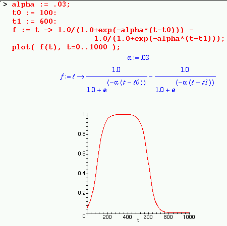
A source of heat within the domain is assumed to exist. This source of heat may depend on time.

Parabolic PDEs Solution

 A finite difference scheme is applied to solve the diffusion equation. First, discretization of the domain is performed. We use h_x = h_y = h = 0.01 and dt = 0.0002 to perform this discretization.  We use a rectangular domain with N_x ~ 2 N_y to acomodate the shape of the source. In what follows, i and j will specify x and y respectively, while the superscript k will specify the time slice.

This diffusion PDE  is written in finite difference form as

(u ^k+1 _ij - u^k_ij ) / dt  = 

       1/2 ( δ²_x u ^k+1 _ij  + δ²_y u ^k+1 _ij + δ²_x u ^k _ij + δ²_y u ^k _ij )   +  1/2 ( S ^k+1_ij + S^k_ij )

where

δ²_x u ^k+1 _ij  =  (   u ^k+1 _{i+1 j} - 2 u ^k+1 _ij + u ^k+1 _{i-1 j} ) / h²

and the same for the time slice specified by k. Let r = dt / ( 2 h ² ). The terms at time k+1 are separated from those at time k to yield

( 1+4r ) u ^k+1 _ij -

           r (  u ^k+1 _{i+1 j}  + u ^k+1 _{i-1 j} + u ^k+1 _{i j+1} + u ^k+1 _{i j-1}) = d ^k _ij

where

d ^k _ij = r (  u ^k _{i+1 j}  + u ^k _{i-1 j} + u ^k _{i j+1} + u ^k _{i j-1}) +

These equations form a linear system of equations for u ^k+1. These are solved iteratively for each time slice.  The lattice is swept repetitively, solving for u ^k+1 _ij  until convergence is obtained. 

u ^k+1 _ij =  (  r (  u ^k+1 _{i+1 j}  + u ^k+1 _{i-1 j}  + u ^k+1 _{i j+1} + u ^k+1 _{i j-1})  +

Serial Implementation

Download the tar file Diffusion_2d.tar containing a directory structure on any serial computer where you can use VisIt. Expand it via:
tar -xvf Diffusion_2d.tar

The directory Difusion_2d contains two directories: diffusion and source.

The code 2d_diffusion.c in the directory diffusion implements the above scheme to solve a 2D diffusion problem. The steps in the code are:

• Initialize the numerical grid and set the boundary values 
• Provide the initial field values
• Set the source term
• Loop over time
• Iterate the solution until convergence at each time step
• Store the field data every so often in time, whereby allowing to make a "movie" post-mortem

The code is compiled and executed via

        gcc 2d_diffusion.c -lm -o 2d_diffusion

        ./2d_diffusion    N_x   N_y  

where N_x and N_y are the (arbitrary)  number of grid points - image size; a ratio 2 to 1 is recommended for the grid sizes in x and y directions. Good numbers to use are ( 700 - 400 ). The code defaults to scan over 3500 time steps.

The code 2d_diffusion.c requires visit_writer.c and visit_writer.h with which it links. This package is used to store the field at each specified time slice in VTK file format in a sub-directory movie. VisIt can form a movie out of these files labeled by a frame number.

Notes about the code 2d_diffusion.c:

• The iterative solution is obtained via double sweeps of the lattice for easier numerical solution
• The code is written in the simplest possible way. The main program is modular to show the steps in the algorithm
• The code outputs the resulting temperature field in files labeled by a frame number. These files are written in a sub-directory. The code visit_writer.c writes the data in VTK format.
• The image data is written every so many (10) iterations through the time evolution of the temperature field, thereby allowing the production of a "movie" post-mortem
• Setting SOURCE to 0 solves the diffusion equation with no source
• When a source is included, the code displays the source term

Better code:

The code Diffusion_2d_pipe_python.tar makes the movie via our python utilities. This makes the movie in real time!

The source:

The code 2d_diffusion.c needs the code 2d_source.c found in the sub-directory source. This code generates the source term to include in the equations. The sub-directory source also contains 2d_source_main.c to see the source. It is compiled and executed via

        gcc 2d_source_main.c -lm -o 2d_source

        ./2d_source

The shape of the source is chosen to represent the word "DREXEL". This word is discretized  in the function drexel_name() to occupy a good fraction of the domain. The shape of each letter is 1 pixel large. This shape is then enlarged via a smoothing procedure (function smooth_text() ). This is done via a simple sum of the neighboring points adjacent to each pixel in the interior domain. This produces the following source geometry ( in a 200 x 100 grid case )

Smoothing passes are repeated to obtain the desired widths for the source ( 4 times in the code ). The function see_image() displays the source geometry ( image above ).

A time dependence is introduced in the code. A graphical representation (through Maple) follows: