
Molecular Dynamics aims at describing the properties of an assembly of molecules in term of their structure and the microscopic interactions between them. It is an extremely powerful numerical approach to describe many-body systems.
Examples of Molecular Dynamics applications abound. For instance, bio-molecular simulations, complex fluids models, crystal models, descriptions of defects in crystals, models of surfaces ... all use variations of Molecular Dynamics. Each of these applications comes with its own set of issues.
The folding of proteins into their native geometrical configurations are often simulated by Molecular Dynamics. The model may assume a chain of beads, the amino acids sequence, surrounded by hundreds or thousand of water molecules. The interactions between the beads themselves and between the beads and the water molecules are adjusted phenomenologically. Newton equations, defining a system of ODEs, are solved numerically. The simulation can be done at constant energy, or at constant temperature using statistical physics concepts. The rotations of the particles (amino acids and water molecules) can be incorporated in the simulation with interactions that depend on the orientation of the molecules in the system. Boundary conditions can be reflexive (to model the containment of a vessel) or periodic to imitate an infinite system and reduce surface effects.
In Ab Initio Molecular Dynamics calculations the molecules are broken into individual atoms. In the Protein Folding problem, the amino acids can be described in terms of individual atoms. The same could be done for the water molecules. Incorporating the individual atoms and chemical bonds leads to more realism. Quantum Mechanics should eventually be used (at an extremely high computational cost) for ultimate reality.
A Simple Code
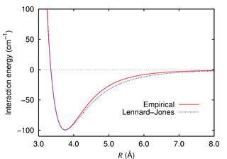
Learning about Molecular Dynamics is best achieved by looking at an example. The code Nbody_basic_verlet.c provides such an example. It solves the problem of N particles that interact via a two-body potential of finite range. Newton equations are solved. The masses are allowed variability. The 2-body interaction is of Lennard-Jones type, the 6-12 potential.
where
The code implements the following steps:
The two-body potential dictates the RHS of the ODEs. Recall
that
![]() . This yields
. This yields
where
Note that the RHS of the ODEs are expensive to compute!
The Basic Verlet ODE integration scheme is used in the code to ensure constancy of the conserved quantities, i.e., energy and momentum. The interpretation of the results and the analysis of the solution rely on maintaining the conserved quantities.
Exercises
The trajectory definitely looks different than for ![]() .
Poincare said that N-body systems with
.
Poincare said that N-body systems with ![]() and larger
are non-integrable (chaotic).
and larger
are non-integrable (chaotic).
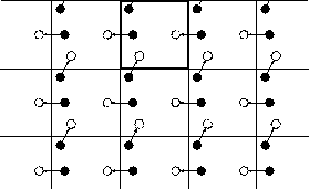
Periodic Boundary Conditions
Some particles in the simulations for ![]() may take off.
They will boil-off following a close encounter (collision)
with other particles through a boomerang effect.
For instance, Molecular Dynamics simulations
of proteins will lead to an explosion of the molecules unless
the relative amino acids positions are
constrained externally or water
molecules are included.
may take off.
They will boil-off following a close encounter (collision)
with other particles through a boomerang effect.
For instance, Molecular Dynamics simulations
of proteins will lead to an explosion of the molecules unless
the relative amino acids positions are
constrained externally or water
molecules are included.
Boundary conditions can also constrain the particles in a finite volume. Reflexive surfaces model a confinement vessel. This approach should be used in gas models where the pressure needs to be calculated.
Periodic Boundary Conditions (PBC) model an infinite system via a finite volume. This is achieved by a cell tiling of the space while including one cell in the calculation. When a molecule escapes through a face of the basic cell, its mirror molecule reappears on the opposite face with the same velocity. This model is equivalent to a basic cell surrounded by image cells.
Code Improvements
The code 'Nbody_basic_verlet.c is to be considered at most as a skeleton of a Molecular Dynamics code. Many aspects of it should be improved. In particular:
Exercises
WEB references
Wikipedia: MD
MD primer
Wikipedia: Periodic Boundary Conditions