The Lorenz Model

The model

   

The Lorenz Model was put forward by Lorenz in 1963 as a simplified model of the convective movements in the atmosphere in the context of weather forecasting. This model was the first model that exhibited chaotic type motion and initiated a new era of studies in nonlinear dynamics. The model made it very evident that the solutions that exhibit chaos depends sensitively on the initial conditions as it happens in weather forecasting.

The model is very nicely described in the book NonLinear Dynamics: A Two-Way Trip from Physics to Math by Solari, Natielo and Mindlin.

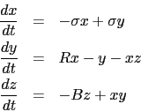
The model is summarized by three coupled first order ordinary differential equations in a three dimensional phase space labeled $x(t)$, $y(t)$, $z(t)$. The equations governing this system are the following:

$$\begin{eqnarray*} \frac{dx}{dt} & = & - \sigma x + \sigma y \\ \frac{dy}{dt} & = & R x - y - x z \\ \frac{dz}{dt} & = & - B z + x y \end{eqnarray*}$$

From our point of view of solving ODEs this problem is quite simple. We use the Runge-Kutta fourth order to solve the equations subject to given initial conditions. What is remarkable about this system is the complexity of the solution that follows.

The code lorenz.c solves the Lorentz model.

   

The Lorenz Attractor

   

The values of the parameters, $\sigma = 10$, $B = 8/3$ and $R = 28$, given as default in the code above, were found by Lorenz in 1963 to generate a chaotic solution. Plotting $x(t)$, $y(t)$, $z(t)$ in 3-dimension (using the gnuplot command splot) displays the very famous butterfly picture of the Lorenz attractor that you find in every textbook. The two-dimensional projection plots, Y vs. X, Z vs. X, and Z vs. Y, are also illustrative of the attractor.

Note that the chaos is exhibited by the solution in going from one spiral to the other one in the butterfly figure.

Plot $x(t)$ vs. $t$. You will see a very rapid motion from left to right on the attractor as exhibited by the curve going from an upper value to a lower value. There is no repetitive pattern to be encountered in this time series.

The Lorenz attractor is a chaotic attractor; it is a fractal. Being an attractor implies that initial trajectories starting from initial conditions in different locations in phase space all converge to it. This is why this arbitrary initial condition that you have seen in the image above leads to the chaotic attractor. The trajectory follows a transient then latches onto the chaotic attractor.

Here is how we can illustrate that and at the same time form a much better image of the Lorenz attractor. Integrate the Lorenz model for a scale time of 100. Store the trajectory into a file. Restart the Lorenz integrator with the - i option to specify X, Y, Z initial as the last X, Y, Z values generated in the previous run over a 100 time scale unit. Run this trajectory for another scaled time of 200 units. Plotting the data in three dimension will produce a sharp image of the Lorenz attractor.

There exist unstable periodic orbits within the Lorentz chaotic attractor. Naturally these are hard to find since they are unstable. We saw in class that the procedure by Henry, Watt, Wearne that uses a lattice refinement scheme to find periodic orbits could be applied to the Lorenz model. Let's illustrate the point that there exists such orbits in a chaotic attractor.

• Integrate the Lorenz model for a scale time of 10 units starting with the initial condition ( x, y, z ) = ( 2.147367 -2.078048 27.0 ) and store the data in a file.

• Integrate the Lorenz model for scale time interval of 10 units starting from the initial condition ( x, y, z ) = ( 4.250440 1.008479 27.0 ) and store the data.

• Plot the two trajectories in three dimensional phase space.

• Plot the Lorenz attractor together with the two trajectories that you just generated. Note that these two trajectories are lying on the attractor.

This illustrates the fact that these trajectories which are periodic unstable orbits are part of the dynamics that drive the establishment of a chaotic attractor.

   

plot3d.c

    

The limit cycles, the Lorenz attractor and the unstable periodic orbits within it are all objects in three dimensions. Wouldn't it be nice to rotate these objects in space to better appreciate their structures. Or equivalently we could rotate the observation point.

The code plot3d.c uses gnuplot to display three dimensional data sets from a rotating observation point. Download the code, run ./plot3d -h and use the three hills potential used in our scattering studies, potential.dat , as a sample data set to practice with.

Use the code to display the three dimensional Lorenz attractor and various periodic orbits.

    

     

A movie!

     

The Lorenz attractor is an extremely complicated object. To further develop one's instinct about how this attractor is built, it is interesting to follow graphically the time evolution of a trajectory that spans the attractor. This is illustrated in the two methods that follow. Note the syntax and the use of LINUX utilities in these two approaches.. In both cases, the trajectory is re-drawn for an ever increasing number of points as generated by our solution of the Lorenz ODE's via rk4. These graphs form a movie when seen in succession.

   

Method 1

The scripts gnuplot_script_1 and gnuplot_script_2 are two GNUPLOT scripts. They assume that the data to span the Lorenz attractor is in the file butterfly. The GNUPLOT graphs are generated by "loading" gnuplot_script_1 via the command load gnuplot_script_1 from GNUPLOT. The looping over the movie frames is generated by gnuplot_script_2 when it loads itself again and again in GNUPLOT, tthereby ``replotting'' the trajectory with an increasing No of points.

The scripts are in movie_gnuplot.tar

Method 2

A mix of a bash shell script and a GNUPLOT script is used to generate a GIF animated ``movie'' from frames containing GNUPLOT graphs. The method reads the trajectory data from the file butterfly. It requires an empty sub-directory movie_frames. It is launched via running bash_script. The script then writes a GNUPLOT script to generate the movie frames in movie_frames in PNG format, converts these to GIF format using the command convert, removes the PNG files and finally (after looping over the frammes) uses gifsicle to merge these GIF files in an animated GIF file in the file anim.gif. The latter can be viewed via ImageMagik commands or via Firefox.

The scripts are in movie_ImageMagik.tar

References

Wikipedia

Serious General Non-Linear Dynamics book by Solari, Natiello and Mindlin

Paper ( local copy ) by Nicholas Report

Nice history of the model

Amazing Pictures