Programs--scientific ones, at least--tend to generate lots of data. You have already seen examples of this in the C-language primer document, and you will see many more. Once, you had little choice as to what you could do with those data. You could only print it out and look at it in the form of columns of figures on the screen. Pretty dull...!
Often, the best way to represent a large dataset is in graphical form. At its simplest, this may just mean drawing simple line graphs. In more sophisticated contexts, you may end up making an elaborate 3-D movie, complete with audio track, to illustrate the Physics and explain your findings to others. Such sophisticated visualization is more an art than a science, and usually calls for specialized hardware and software (although you can actually get quite far without leaving our lab). Here, we will confine ourselves to a discussion of a few basic programs and packages to help you make simple plots and images from your data.
The following is a list of some useful graphics tools available on our system:
| simple_plot: | a minimal collection of graphics routines, for use within a user's C program |
| plot_data: | a simple pipelined line-drawing program |
| gpl: | an even simpler pipelined line-drawing program, based on gnuplot (see below) |
| mcdraw: | not so easy to use, but more powerful, mostly 2-D line-drawing package. |
| gnuplot: | a very powerful 2-D and 3-D plotting package. |
| make_image: | simple program to convert data into images |
| make_images: | simple program to convert a stream of data into multiple images |
| convert: | useful routines to convert one image format into another |
| gifsicle: | turn a collection of GIF images into an animation! |
| png2mng: | same, for PNG images |
Many others exist, but these will be sufficient for our purposes.
#include <stdio.h>
#include <math.h>

#define N_POINTS 1000
#define XMIN 	 0
#define XMAX 	 (4 * M_PI)	/* this is just 4 PI; M_PI defined in math.h */

main()
{
    int i;
    double x;

    for (i = 0; i < N_POINTS; i++) {
	x = XMIN + i * (XMAX - XMIN) / (N_POINTS - 1);
	printf("%f %f %f\n", x, sin(x), cos(x));
    }
}
This will produce 3 columns of data, with 1000 rows in each, listing
the values of x, sin x and cos x, for values of x linearly spaced
between 0 and 4 PI.In the simplest possible case, to draw a graph of, say sin x versus x (column 2 versus column 1), we must do the following:
The following functions are declared in the header file simple_plot.h. To use these functions, include simple_plot.h in your C program and compile using the system ``Cgfx'' command, which will find the proper header files and use the correct graphics libraries.
void draw_box(float xmin, float xmax, char *xlabel, float ymin, float ymax, char *ylabel); | initialize graphics and draw a box with axes running from xmin to xmax in x and ymin to ymax in y, with labels as specified (label = NULL ==> no label drawn) |
void add_label(char *label); | add an overall label centered above the box |
void set_color(char *color); | specify the (standard X) color used for all subsequent graphics operations |
void plot(float *x, float *y, int n); | plot the array y as a function of the array x, plotting only those points lying within the box |
void move_to(float x, float y); | move to (x, y) |
void draw_to(float x, float y); | draw to (x, y), showing only the portion of the line lying within the box |
void point(float x, float y, float size); | draw a ``point'' at (x, y), with size specified in x-axis units |
void get_mouse(float *x, float *y); | return the current position of the mouse (wait for right mouse button to be pressed) |
int check_mouse(); | return 0 if no mouse button has been pressed, the number of the mouse button (1=L, 2=M, 3=R) otherwise (no waiting) |
void wait_for_mouse(); | wait for a mouse button to be pressed, then return |
void pause(int time); | pause for 'time' microseconds |
void clear_graphics(); | erase the entire display |
void exit_graphics(); | quit the graphics package |
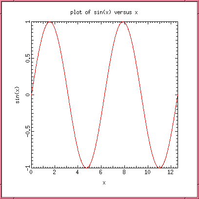
Thus, to perform the actions listed above for the sine function, we can use the following program:
#include <stdio.h>
#include <math.h>

#include "simple_plot.h"

#define N_POINTS 1000
#define XMIN 	 0
#define XMAX 	 (4 * M_PI)	/* this is just 4 PI; M_PI defined in math.h */

main()
{
    int i;
    double x;

    set_color("black");		/* (this is the default) */

    draw_box(XMIN, XMAX, "x", -1, 1, "sin(x)");
    add_label("plot of sin(x) versus x");

    move_to(XMIN, sin(XMIN));
    set_color("red");
    for (i = 0; i < N_POINTS; i++) {
	x = XMIN + i * (XMAX - XMIN) / (N_POINTS - 1);
	draw_to(x, sin(x));
    }

    exit_graphics();
}
The result should look something like:

An alternative, and in many ways simpler, approach is to use the ``black box'' plotting program plot_data, described below, which contains within it all the knowledge needed to make fairly complete plots on an X-window display. The program itself makes calls to the lux interface library written by ex-Drexel graduate student Biao Lu. If you are interested in seeing what is involved in dealing with X at this level, look in the plot_data and lux source code (distributed as part of the ``Starlab'' software package). In fact, the simple_plot library functions are identical to those used by plot_data.
The plot_data program accepts as input columns of data in character, integer, or floating-point format. It selects two columns, then performs all the operations listed above to produce a graph on the X-terminal. If the above program (producing x, sin x and cos x) has been compiled and called trig, then we can plot a graph of sin x simply by typing
trig | plot_dataYou should see something like:
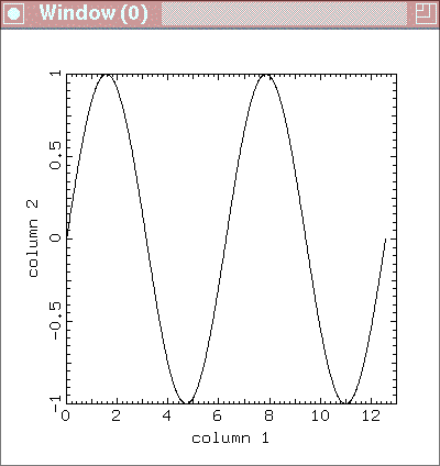
By default, plot_data plots column 1 as the x (horizontal) axis, column 2 as the y (vertical) axis. Its defaults are selected so that it does something ``reasonable'' with the minimum of user input.
Suppose we want a graph of cos x instead. To specify the columns to plot, use the command-line switch -c xcol ycol. This will result in xcol being plotted as x, ycol as y (so the default is xcol = 1, ycol = 2). Thus, we would say:
trig | plot_data -c 1 3The graph will now look like:
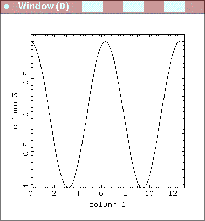
By default, the limits on the x and y axes are taken from the data. To override this and set your own, use the -l xmin xmax ymin ymax switch, which forces the range on the x-axis to be [xmin, xmax] and that on the y-axis to be [ymin, ymax].
There are several more options to allow you to control the appearance of your graph. Here is the complete list.
        -c xcol ycol1 ycol2 ycol3...
                        plot data in xcol horizontally, ycol1, ycol2,
			ycol3,... vertically [1 2]
        -c[c][xy]       crop [x or y] data to plot limits
        -C color1 color2 color3...
                        specify line/point colors for the columns set
			by "-c" [all black]
        -e              echo current settings
        -h header       specify overall label for plot [none]
        -i              ignore inline commands [don't ignore]
        -l xmin xmax ymin ymax  specify limits for plot [get from data]
        -ll             force plot lines only [plot lines]
        -L scale        specify limits to be +/- scale for both axes
        -N nmax         specify maximum number of points to store [50000]
        -o              echo stdin to stdout [do not echo]
        -O xo yo        specify top left corner of plotting box [150, 50]
        -p              toggle plot points only [plot lines]
        -pp             force plot points only [plot lines]
        -P size         specify point size, in x-axis units [0 ==> pixel]
        -q              suppress most output [don't suppress]
        -Q              quit
        -s xs ys        specify box size [500, 500]
        -S skip         skip leading lines [0]
        -t ntrail       specify number of trailing points [infinite]
        -w[w][xy]       wrap [x or y] data to plot limits
        -W              wait for keyboard input [inline only]
        -x xlabel       specify label for x-axis ["column 'xcol'"]
        -X              clear the display and redraw axes [inline only]
        -y ylabel       specify label for y-axis ["column 'ycol1...'"]
        -z zcol         specify column for color data [none]
The expressions in square brackets are the defaults. To get this
list, you can type plot_data --help.Most of the above options are fairly self-explanatory. One useful feature of the program is that it can read in several columns of data, and plot the first on the horizontal axis, all the others vertically. The -C option allows each graph to be plotted in a different color (specified as standard X color names -- red, blue, green, etc.), if desired.
Alternatively, plot_data can read in three columns of data (x, y, and z, say) and plot y against x, choosing the color of each point according to the value of the data in z. The mapping between z-value and color is presently fairly rudimentary, but improvements are in the works.
The limits for the graphs may be specified on the command line, in which case plot_data draws the axes first and plots points as they become available, allowing you to see the plot evolve, or to make animations (-t option). Otherwise, plot_data must determine the limits from the input data, so nothing is plotted until the entire data stream is read.
Some examples (assume that the program data produces the stream of data to plot):
data | plot_data -c 3 2 7 -C red green -x X -y Y -l -1 1 0 1
data | plot_data -p -C red
data | plot_data -c 4 5 -s 800 800 -z 7
Finally, the current version of plot_data accepts most of the above command-line options as embedded commands in the input data stream itself, allowing the user to exercise run-time control over the display. For example, if the command line indicates that a single column is to be plotted in the vertical direction, and that the data are to be plotted as lines, then if the data stream contains
        .
        .
        .
        x  y  z
        x  y  z
        x  y  z
	-C red -p
        x  y  z
        x  y  z
        .
        .
        .
the effect of the inline command will be to switch the plot color to
red and to enter point mode. Subsequent commands might clear the
screen, redefine the axes, change the size of plotted points or the
number of points plotted in ``trail'' mode, and so on. All commands
except -i, -N, -o, and -s
are inlinable. In addition, some commands only operate in inline
mode: the pause (-W) option allows the program to wait for
a keyclick from the user before continuing; and the -X
command clears the display and redraws the axes.
In order to to use inline commands, it is necessary that a window be opened for plotting at the start of input, not at the end, and this requires that some scaling information be provided on the command line. (If no such information is avaliable, then plot_data must obtain limits from the data, so the entire graph is drawn after the data are read and inline commands are ignored.) However, since the limits themselves can be set by inline commands, all that is really necessary is for plot_data to be forced to open a window, so a simple command like
plot_data -Lwill suffice (the default for -L is 1). True limits, labels, graphs, colors, etc. can then be specified by the program producing the data. For example, the plot produced by the first example above could also be created by having the program data print out the line
-c 3 2 7 -C red green -x X -y Y -l -1 1 0 1before printing its output, and typing
data | plot_data -Lon the command line. This simple technique allows a user to write remarkably complex graphics programs using nothing more sophisticated than printf statements!
xwd | xpr | lpror possibly
convert x: ps:- | lprYour cursor will turn into a cross and you will click in the (plot_data) window you want to plot; xwd then creates an X-window dump (bitmap) of the window, xpr converts it to PostScript, and lpr prints it. In the second form, the convert program (available on many systems) converts an X window directly into PostScript. In either case, since the printout is a bitmap scaled to the size of the printed page, the best resolution will be obtained by making the plot_data window as large as possible before printing.
Unlike plot_data, mcdraw prompts the user for all input data -- filenames, columns to plot, output device (which doesn't have to be an X-display), and so on -- then draws the graph and waits for more input. Its original purpose was to produce publication-quality plots in a simple fashion. As a result, it has better fonts and heuristics for deciding what ``looks right'' than exist in plot_data. However, it has expanded in scope over the years, and can now do quite sophisticated operations, such as data reduction, array arithmetic, curve fitting, among others.
A typical mcdraw session, to produce a plot similar to the first example shown above, might look like:
	mcdraw:	file DATA	# open a data file called DATA
	mcdraw:	c 3 2		# get x from column 3, y from column 2
	mcdraw:	lim -1 1 0 1	# set limits on x and y
	mcdraw:	de x		# initialize graphics in X-windows
	mcdraw:	xl X		# specify the x-label as "X"
	mcdraw:	yl Y		# specify the y-label as "Y"
	mcdraw:	box		# draw a box, with labelled axes, etc.
	mcdraw:	plot		# plot y(x)
	mcdraw:	la LABEL	# put an overall label ("LABEL") on the figure.
	mcdraw:	quit		# exit from MCDRAW.
The ``#'' means that the rest of the line is a comment. Commands may
be ruthlessly abbreviated and combined on a single line, separated by
semicolons, so the above command sequence could be equally well
written as:
mcdraw: f DATA; c 3 2; l -1 1 0 1; de x; xl X; yl Y; b; p; qFor more information on mcdraw and a complete description of the present command set, see the mcdraw primer.
One possibility is just to make contour plots of the ``level lines'' of the dependent function f. mcdraw has a ``2d'' mode which will allow you to do this interactively. A second possibility is to make three-dimensional perspective plots of the surface in (x, y, z space) defined by z = f(x, y). mcdraw can do this too, in a fairly primitive manner. A much more sophisticated 3-D plotting package is khoros, a public-domain X utility.
A very commonly used technique for displaying two-dimensional data is to make an image. This has the considerable advantage of enlisting the assistance of the many image-display and image-processing programs that exist in the public domain. In addition, images can be easily combined to make movies using the mpeg_encode program.
On our systems, the color resolution of our screens allows us to display up to 256 colors simultaneously. The number is chosen because integers in the range 0 to 255 can be represented using a single byte of data--an unsigned char in C. Of course, there are many ways to choose these colors. The mapping between the integers 0 to 255 and the final color that appears on the display is called a color map. The standard color map we use looks like this:

There is no particular reason for this choice--it is simply convenient. Small numbers correspond to blue, large numbers to red, and intermediate numbers to intermediate colors in the ``spectrum''. The programs mcdraw and make_image (described in a moment) allow you to change the color map to one of your own, if you so desire.
To X, an image is a collection of bytes, one per pixel, along with a color map telling the display how to ``paint'' the screen. There are many different image formats in use--gif, jpeg, miff, xpn, to name but a few. Fortunately, we don't have to know how to construct them all. The program convert allows us to turn one into another.
To assist in turning your data into an image, we have provinded a simple program called make_image. This program takes a stream of data (fdrom stdin) representing your image (scanned left to right, top to bottom), adds a header describing the color map (the standard one, by default), and writes the image to stdout. The data may be float (the default), int, or char, and are assumed already to be scaled to lie in the range 0 to 255. Thus, to make a simple image, assuming that data produces the correct input, just type:
data | make_image -s XSIZE YSIZE > imageYou must specify XSIZE and YSIZE to tell the make_image how to divide the data string up into rows. The file image produced in this way may be viewed with xv or display.
The file created my make_image is in so-called ``Sun rasterfile'' format. This format has no particular advantage, except that it is simple and easy to code. To make, say, a GIF file, use convert:
convert image image.gifYou can also do the conversion in a pipe without creating an intermediate Sun rasterfile:
data | make_image -s XSIZE YSIZE | convert - image.gifThe full list of make_image options is:
	-c	  incoming data are in char form
	-i	  incoming data are in int form
	-f	  incoming data are in float form [default]
	-m file	  read the colormap from the specified file
	-p	  pad the image to even dimensions (Sun rasterfile limitation)
	-s m n	  specify the dimensions of the image to be m by n
		  If only m is given, take n = m
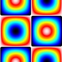
The following simple program produces some sample image data
#include <stdio.h>
#include <math.h>

#define N_POINTS 200

main()
{
    int i, j;
    double x, y;

    for (j = 0; j < N_POINTS; j++)
	for (i = 0; i < N_POINTS; i++) {
	    x = 2*i*M_PI/N_POINTS;
	    y = 2*j*M_PI/N_POINTS;
	    printf("%f ", 255*(1 + sin(x)*cos(y)));
	}
}
Compile this as data, then type
data | make_image -s 200 | xv -and you will see:
-F name set the "base" name for image fileswhich defines the base name to be used in naming the output files. The default is "IMAGE", and successive images are saved in files IMAGE.0000, IMAGE.0001, etc.
Thus, if the program data produces a stream of image data in the form of 200x200 arrays, typing
data | make_images -s 200 -F TEMPwill create a series of files TEMP.0000, TEMP.0001,... containing Sun rasterfile images derived from the input data. New image files will continue to be created until the input data stream terminates.
The image files may be conveniently viewed using the animate utility by typing
animate TEMP.*