


Next: Elementary quantization of the
Up: The Hermite Polynomial &
Previous: The Hermite Polynomial &
Hooke first discovered the law of springs, that their force is
proportional to their displacement. In reality, their force is
generally a far more complicated function. In fact, many complicated
forces can be approximated in a form similar to the harmonic oscillator.
Consider the potential  describing some physical phenomenon. Close
enough to the equilibrium point x=a, we can expand this function as a Taylor
polynomial,
describing some physical phenomenon. Close
enough to the equilibrium point x=a, we can expand this function as a Taylor
polynomial,
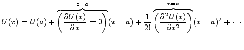 |
(1.1) |
Here the first derivative is zero, as we take the Taylor series around an
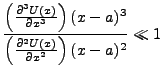
equilibrium. How close is close enough? This would depend on the degree of accuracy one
seeks, though generally it is assumed that
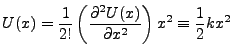
We are at liberty to rescale our potential so that  , whereby we have the approximation,
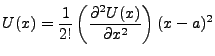 |
(1.2) |
It is typical to also rescale the x-axis so that  and, using common terminology,
Here k is a constant. The equation of motion for such an object becomes
and, using common terminology,
Here k is a constant. The equation of motion for such an object becomes

typically

Often it is more accurate to add a damping term, for example, a spring
under water is better described by,
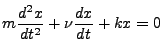 |
(1.3) |
Here  is some constant defined by the retarding
force
is some constant defined by the retarding
force
 . If a harmonic driving force is
applied, Equation 1.3 becomes inhomogeneous,
. If a harmonic driving force is
applied, Equation 1.3 becomes inhomogeneous,
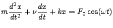 |
(1.4) |
Equation 1.3 is easiest to solve. Let
 ,
,
 , and
, and
 . If we suppose the solution
 ,
,
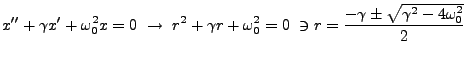 |
(1.5) |
We seek a fundamental set of solutions to these equations. From the theory of
differential equations we know that we require exactly two distinct solutions.
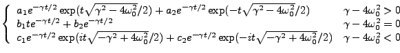
The  in the solution to the characteristic equation lends us two such
solutions, except in the case when
in the solution to the characteristic equation lends us two such
solutions, except in the case when
 .
In that case, our first solution is
.
In that case, our first solution is
 |
(1.6) |
The characteristic equation suggest no further solution. The method of reduction
of order has us assume that
 |
(1.7) |
Plugging Equation 1.7 into Equation 1.5, we find that  and so
The Wronskian of these two solutions is nonzero always, and so we have
a fundamental set of solutions. The other cases are more easily solved
and we find,
and so
The Wronskian of these two solutions is nonzero always, and so we have
a fundamental set of solutions. The other cases are more easily solved
and we find,
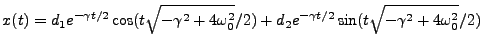
The latter can be written,
The driven Equation (1.4) is slightly more complicated to solve.
In Equation 1.4 one can replace
 with
with
 on the condition we take the real part of the
solution to be found from this ``axillary equation'' [2]. If we suppose a solution
on the condition we take the real part of the
solution to be found from this ``axillary equation'' [2]. If we suppose a solution
 ,
we find,
,
we find,
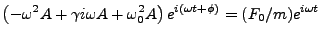 |
(1.8) |
Dividing out the exponent on the left hand side and equating real and imaginary
parts of the right yields,
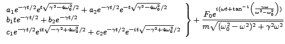
The full solution to the driven damped harmonic oscillator is then,
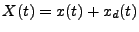 |
(1.9) |
Here x(t) is the solution to the homogeneous equation we found above (one of the three variations
depending on the parameters). Or, since we enjoy seeing large equations in their full forms,
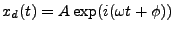
Figure 1.1:
Examples of three possible solution types for the homogeneous damped harmonic equation.
|
|
Next: Elementary quantization of the
Up: The Hermite Polynomial &
Previous: The Hermite Polynomial &
Timothy D. Jones
2007-01-29

![\includegraphics[width=10cm]{harm1.ps}](img36.png)