


Next: Theoretical Example of Decoherence
Up: Is Quantum Decoherence the
Previous: Theoretical Example of Superposition
Contents
A review of an experiment in which superposition is demonstrated follows. We focus specifically on work done
by the Laboratoire Brossel in Paris [3,4,1]. In their experiments using Ramsey interferometry,
a microwave cavity, and an ensemble of Rydberg atoms, the Paris team not only demonstrate quantum superposition,
but they were also able to demonstrate decoherence. The reader curious for more detail than presented here
is especially encouraged to read the theoretical proposal of Davidovich et al. [3].
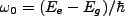
The experimental set up is shown in Figure 3.1. A resonant cavity (C) is prepared to contain
a field off resonance with the
 resonance , though for the following two examples this cavity is inactive (but plays
a crucial part in the decoherence experiment). The Paris group uses a high-Q cavity, where
resonance , though for the following two examples this cavity is inactive (but plays
a crucial part in the decoherence experiment). The Paris group uses a high-Q cavity, where
 , is a measure
of the efficiency of the cavity in storing a field (
, is a measure
of the efficiency of the cavity in storing a field (
 is the energy stored,
  is the resonant frequency, and
  is the energy loss) such that the average lifetime of a resonant photon in the cavity is proportional to Q [17] and
thus has a relatively long relaxation time. A coherent state is injected from (S) into the cavity (C) in a later experiment discussed regarding decoherence.
is the energy loss) such that the average lifetime of a resonant photon in the cavity is proportional to Q [17] and
thus has a relatively long relaxation time. A coherent state is injected from (S) into the cavity (C) in a later experiment discussed regarding decoherence.
Two low-Q cavities are used (R1, R2) to apply microwave fields produced by S'. B represents a ``black-box'' which prepares Rydberg
atoms (atoms with one valence electron in an extremely high n state), and (De) and (Dg) are detectors which provide
an electric field that is sufficient to ionize the Rydberg atoms in their excited state (De) or ground state (Dg).
Laser beams L1, L1' are used to select for atoms of the proper velocity, and the L2, B setup excites Rydberg atoms into
their circular states (high quantum number n). The entire setup is enclosed and cooled to 0.6K to make thermal radiation negligible.
Figure 3.1:
Experimental setup from [1] Paris group (1996)
|
|
Henceforth we shall assume ideality and ignore experimental details which detract from the flow
of our report. The actual experiment followed closely. The Rydberg atoms are excited into the states  or
or  corresponding
to quantum number
corresponding
to quantum number  and
and  respectively. The
 transition
frequency is 51.099 GHz [3], and cavities R1 and R2 contain fields resonant with this transition.
transition
frequency is 51.099 GHz [3], and cavities R1 and R2 contain fields resonant with this transition.
To describe what happens to the atom as it passes through R1 toward C and R2, we need to introduce (briefly)
the semi-classical Rabi model [7] appropriate for such resonance. The derivation is simpler
in the semi-classical form, but similar results can be obtained (see appendix) in the full quantum (i.e. Jaynes-Cummings model)
derivation. Furthermore, it can be demonstrated that the fields in R1 and R2 behave classically and so do not produce entanglement,
thus justifying a semi-classical approach [18].
We assume an atom capable of being in two states (a good approximation for a Rydberg atom under controlled
circumstances),
and
where
 and the laser field produces a frequency
 .
We assume an interaction Hamiltonian of simply
.
We assume an interaction Hamiltonian of simply
 . The state vector can be written,
 |
(3.1) |
Using the time-dependent Schrödinger equation gives
A valid assumption has us suppose that  and
and  , and using the
identity
, and using the
identity
 , we make application
of the ``Rotating wave approximation'' where terms
, we make application
of the ``Rotating wave approximation'' where terms
 are disregarded
and terms
are disregarded
and terms
 are kept (since
  is in near resonance, this latter
term dominates the behavior),
is in near resonance, this latter
term dominates the behavior),
Here
 is called the detuning of the atomic transition frequency and
laser field. After assuming a characteristic solution of
is called the detuning of the atomic transition frequency and
laser field. After assuming a characteristic solution of
 we arrive at a
characteristic equation of
we arrive at a
characteristic equation of
 ,
and fitting the given initial conditions, one finds,
,
and fitting the given initial conditions, one finds,
To introduce the concept of  and
and  pulses, we consider the case when
  .
Then
.
Then
Define the atomic inversion as
 . Thus we see how
the probability of an atom exposed to a resonant field being in one state or the other is
dependent upon the time exposed to the field. We make this explicit in the following table.
. Thus we see how
the probability of an atom exposed to a resonant field being in one state or the other is
dependent upon the time exposed to the field. We make this explicit in the following table.
Pulse

|
:

|
:

|
| W(t) |
1 |
0 |
| Status |
 ,
, 
|
 ,
,

|
Thus we see the necessity for monokinetic Rydberg atoms (though in actuality one gets
quasimonokinetic Rydberg atoms [3]). The speed of the atoms will determine
their time exposed to the  and
and  fields, and thus the state function.
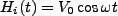
In order to obtain the statistics necessary to make quantum mechanical measurements,
we desire the ability to nearly perfectly replicate the initial state (the state preparation
procedure). The Paris group demonstrated this ability and the Rabi oscillation in 1995 [5]
under a similar but simpler apparatus shown in Figure 3.1. They repeat the state
preparation on a large set of Rydberg atoms, select those of a certain speed which will
result in a corresponding exposure time to the resonant field, and record the the state
of the atom after exiting the field. For each selected t, about 20,000 are measured and
their state probability (
fields, and thus the state function.
In order to obtain the statistics necessary to make quantum mechanical measurements,
we desire the ability to nearly perfectly replicate the initial state (the state preparation
procedure). The Paris group demonstrated this ability and the Rabi oscillation in 1995 [5]
under a similar but simpler apparatus shown in Figure 3.1. They repeat the state
preparation on a large set of Rydberg atoms, select those of a certain speed which will
result in a corresponding exposure time to the resonant field, and record the the state
of the atom after exiting the field. For each selected t, about 20,000 are measured and
their state probability (
 ,
,
 ) is averaged.
Figure:
Experimental Rabi oscillations from [4,5] Paris group. Initial state is
with a
pulse corresponding to a collective shift to the ground state. The dampening
of the oscillation is due to technical imperfections in the experiment.
|
|
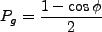
Now let us explore the progress of a Rydberg atom in the larger Paris group experiment. We will follow
one atom, and suppose it starts out simply in the excited state,
 . The atom
has a velocity such that its time through the R1 resonance chamber is a
pulse, and the atom
exits in the state, ideally,
. The atom
has a velocity such that its time through the R1 resonance chamber is a
pulse, and the atom
exits in the state, ideally,
 |
(3.2) |
However, realistically we expect the detuning will be non-zero, which introduces a phase difference,
Here
 where T is the exposure time to the second ``Ramsey'' beam.
We see that the atom has two identical paths for ending up in each of the electronic states,
and thus enters the superposition.
where T is the exposure time to the second ``Ramsey'' beam.
We see that the atom has two identical paths for ending up in each of the electronic states,
and thus enters the superposition.
Figure 3.3:
Possible paths for the wave function.
|
|
The probability of finding the atom in
is thus the squared sum of the amplitude
of the two possible paths, i.e.,
 |
(3.3) |
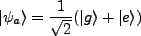
This is exactly what the Paris team found in one such experiment [4]. There result is shown in
Figure 3.4.
Figure 3.4:
Experimental evidence of Ramsey fringes from the superposition of two quantum paths (from [4]). The fringes
have 85% contrast due to various non-idealities in the experimental set-up.
|
|
Thus we have seen both theoretical and real-world examples of quantum effects that must be removed
by decoherence.
Next: Theoretical Example of Decoherence
Up: Is Quantum Decoherence the
Previous: Theoretical Example of Superposition
Contents
tim jones
2007-04-11
![\includegraphics[width=7.5cm]{paris.ps}](img97.png)
![\includegraphics[width=7.5cm]{ram3.ps}](img104.png)
![\includegraphics[width=7.5cm]{ram.ps}](img44.png)
![\includegraphics[width=4.5cm]{ram2.ps}](img102.png)